
Chapter 54
Malus Law and Polarisation Alignment

Wave Coherence and Optics
Author: Mark Anthony Higgins
© Mark Anthony Higgins 11 October 2025
Revised Date: 23 February 2026
Audio Overview
Flow Algebra
flow "Malus Law and Polarisation Alignment" v1.0

# ---------- PURPOSE ----------
# Describes intensity variation due to polarisation angle between light and an analyser.
# Based on Malus’ law: I = I0 cos²θ.
# Expressed as a coherence alignment between electric field orientation and boundary axis.
# IB measures the polarisation coherence (1 = perfect polarisation, 0 = unpolarised).
# IB < 1 introduces partial coherence or mixed polarisation states.

# ---------- PARAMETERS ----------
params:
  units: "SI"
  I0: positive                  # initial intensity [W/m²]
  θ: real                       # relative angle between E-field and polariser axis [radians]
  IB: 0.0..1.0 = 1.0            # polarisation coherence index
  include_partial: bool = false
  λ_decay: nonnegative = 0.0    # coherence loss constant [s^-1]
  dt: positive?                 # timestep for coherence change
  rotation_speed: real = 0.0    # rotation rate of analyser [rad/s]

# ---------- STATE ----------
state Polarisation:
  I: real                       # transmitted intensity [W/m²]
  E_align: real                 # field alignment component (cosθ)
  phase_diff: real              # phase offset between field components
  coherence_loss: real          # 1 - IB
  polarisation_state: str       # "aligned", "partial", or "random"

# ---------- INVARIANTS ----------
invariants:

  # Compute field alignment
  Polarisation.E_align = cos(params.θ)

  # Malus’ law: transmitted intensity
  Polarisation.I = params.I0 * (Polarisation.E_align)^2 * params.IB

  # Phase difference component (for ellipticity or birefringence)
  Polarisation.phase_diff = sin(2 * params.θ) * (1 - params.IB)

  # Coherence decay law
  if params.λ_decay > 0:
    params.IB = clamp(params.IB - params.λ_decay * (1 - params.IB) * (params.dt or 1), 0, 1)
    Polarisation.coherence_loss = 1 - params.IB
  else:
    Polarisation.coherence_loss = 0

  # Polarisation classification
  if params.IB == 1:
    Polarisation.polarisation_state = "aligned"
  elif params.IB > 0.5:
    Polarisation.polarisation_state = "partial"
  else:
    Polarisation.polarisation_state = "random"

# ---------- TRANSFORMS ----------
transforms:

  rotate_polariser:
    comment: "Increment angle θ to simulate rotation of analyser."
    params.θ += params.rotation_speed * (params.dt or 1)
    if params.θ > 2π:
      params.θ -= 2π

  decay_coherence:
    comment: "Simulate depolarisation over time."
    params.IB = clamp(params.IB - 0.01 * (1 - params.IB), 0, 1)

  restore_alignment:
    comment: "Gradually realign field and polariser axes."
    params.θ -= 0.1 * sin(params.θ)

# ---------- MONITORS ----------
monitors:
  malus_consistency:
    assert Polarisation.I >= 0
    comment: "Intensity remains non-negative."
  coherence_bounds:
    assert 0 <= params.IB <= 1
  phase_alignment:
    if abs(sin(params.θ)) < 0.1:
      comment: "Field and analyser axes nearly aligned — maximum transmission."

# ---------- SCENES ----------
scenes:

  perfect_alignment:
    given params:
      I0: 1.0
      θ: 0
      IB: 1.0
    expect:
      Polarisation.I = 1.0
      Polarisation.polarisation_state = "aligned"
      comment: "E-field fully aligned with polariser axis — maximum transmission."

  cross_polarised:
    given params:
      I0: 1.0
      θ: π/2
      IB: 1.0
    expect:
      Polarisation.I = 0
      comment: "Perpendicular polarisation — no transmission."

  partial_polarisation:
    given params:
      I0: 1.0
      θ: π/4
      IB: 0.6
    expect:
      Polarisation.I ≈ 0.3
      Polarisation.polarisation_state = "partial"
      comment: "Mixed polarisation — reduced transmission."

  rotating_polariser:
    given params:
      I0: 1.0
      θ: 0
      rotation_speed: π/8
      IB: 1.0
      dt: 1.0
    enable:
      - rotate_polariser
    expect:
      Polarisation.I oscillates as cos²θ
      comment: "Intensity modulates periodically — dynamic Malus effect."

# ---------- NOTES ----------
notes:
  - **Malus’ Law:**  
    \[
    I = I_0 \cos^2\theta
    \]
    Intensity of transmitted light depends on the cosine of the angle between E-field and analyser axis.

  - **Polarisation Coherence:**  
    \[
    I = I_0 I_B \cos^2\theta
    \]
    where \(I_B\) represents coherence in polarisation orientation (1 = fully polarised).

  - **Coherence Decay:**  
    \[
    \dot{I_B} = -\lambda (1 - I_B)
    \]
    Models gradual loss of polarisation due to scattering or thermal noise.

  - **Interpretation:**  
    - Polarisation represents directional coherence of the electric field.  
    - Malus’ law is not merely a geometric projection but a measure of *alignment of curvature fields*.  
    - \(I_B\) quantifies how well this alignment persists through boundary interactions.  
    - Depolarisation corresponds to coherence diffusion across orthogonal modes.

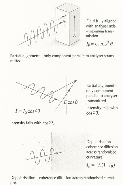
  - **Visualization:**  
    - Left: vector E-field at angle θ to analyser axis.  
    - Middle: transmitted component (E cosθ) through polariser.  
    - Right: partial or randomised field under depolarisation (IB < 1).
Overview

Light is not simply energy travelling through space — it is structured curvature vibrating in orientation as well as amplitude.
When that curvature meets a boundary, only the component aligned with the boundary’s internal coherence can pass.
This angular filtering of curvature is what classical physics calls polarisation.
Malus’ Law quantifies this process through a simple rule of projection, yet beneath it lies a precise geometry of coherence alignment.


🔹 1. Classical Form — Malus’ Law

When a beam of plane-polarised light strikes a polarising filter at an angle θ, only the component of its electric field aligned with the analyser’s axis is transmitted.
The transmitted intensity follows:

\[ I = I_0 \cos^2\theta \]

At θ = 0, the light is fully aligned — maximum transmission.
At θ = π/2, the field is perpendicular — transmission falls to zero.
This rule is purely geometric in form, describing how a vector’s projection determines the observed amplitude.

But the geometry is not external; it is internal curvature projection — the field aligning (or misaligning) its oscillation with the analyser’s boundary orientation.


🔸 2. Coherence Interpretation — Alignment as Boundary Memory

In the coherence framework, the polariser acts as a boundary of directional memory.
It transmits only the field components that remain phase-locked to its own internal axis of curvature.
The relation becomes:

\[ I = I_0 I_B \cos^2\theta \]

where IBI_B is the boundary coherence index, describing how purely the field retains its polarisation structure.

  • IB=1I_B = 1: perfect coherence — single orientation, stable field memory.
  • IB<1I_B < 1: partial coherence — mixed or fluctuating orientations.
  • IB→0I_B \to 0: unpolarised light — random curvature, no preferred direction.

In this view, polarisation is not a mechanical filtering of waves but a coherence selection process:
the field’s alignment with the boundary’s preferred curvature determines transmission.


🔹 3. Phase and Curvature Dynamics

At the vector level, the field can be represented as:

\[ \mathbf{E} = E_0 (\cos\theta\,\hat{x} + \sin\theta\,\hat{y}) \]

A polariser extracts one axis of this curvature, converting the oscillation from two-dimensional rotation to a single-axis vibration.
The lost component does not vanish — its curvature becomes incoherent within the boundary plane, contributing to absorption or scattered radiation.

When partial coherence exists (IB<1I_B < 1), the phase relationship between orthogonal components fluctuates.
This gives rise to elliptically or circularly polarised states, where curvature memory persists but rotates dynamically — a self-modulating boundary alignment.


🔸 4. Coherence Decay — Depolarisation and Boundary Diffusion

Real systems are rarely perfect.
Scattering, reflections, or material anisotropy introduce small phase shifts between orthogonal field components, leading to gradual depolarisation:

\[ \dot{I_B} = -\lambda (1 - I_B) \]

Here, λ\lambda defines the rate of coherence loss — how quickly the field’s memory of direction diffuses into noise.
As IBI_B falls, the polarisation ellipse collapses into randomness, and the transmitted light loses its structural orientation.

In this way, depolarisation is coherence diffusion: the boundary fails to preserve a stable curvature axis.


🔹 5. Unified Boundary Logic — Alignment as Curvature Agreement

Malus’ Law and polarisation are expressions of a deeper rule:
only curvature aligned with boundary geometry can persist coherently through it.
When the field is aligned, the boundary recognises it — transmission is maximal.
When misaligned, the boundary rejects it — curvature coherence is destroyed or reflected.

This same logic underlies all boundary phenomena:

  • Reflection → curvature reversal.
  • Refraction → curvature translation.
  • Polarisation → curvature orientation selection.

In each case, the boundary functions as a curvature filter, enforcing coherence continuity across its surface.


🧠 Summary

Malus’ Law reveals that light’s intensity is a measure of how well its curvature aligns with the boundary’s orientation.
Classically, it describes projection; in the HST–Flow view, it expresses coherence agreement.

  • I = I₀ cos²θ → projection geometry.
  • I = I₀ I_B cos²θ → curvature alignment with coherence retention.
  • I_B → memory of polarisation integrity across time or interaction.

When boundaries and fields are perfectly aligned, light passes in full coherence.
When misaligned, phase memory fragments, and intensity decays.
This is not attenuation by absorption, but loss of structural agreement — the curvature’s memory no longer matching the geometry through which it moves.

In short:

Malus’ Law describes the geometry of coherence itself —
how light remembers the direction of its own oscillation.


Kireth Research
38 Thorndale Croft, Wetwang, Driffield
East Riding of Yorkshire YO25 9XZ
Designed By