Chapter 33
Poiseuille and Stokes Viscous Coherence
Fluid and Mechanical Media
Author: Mark Anthony Higgins
© Mark Anthony Higgins 11 October 2025
Revised Date: 23 February 2026
flow "Poiseuille and Stokes — Viscous Coherence" v1.0
# ---------- PURPOSE ----------
# Unifies laminar pipe flow (Hagen–Poiseuille) and low-Re particle drag (Stokes) as
# expressions of viscous coherence. Introduces a boundary coherence index (IB) to map
# wall/particle slip, micro-roughness, and early transition effects. Blends to Darcy–Weisbach
# form via Re when needed.
# ---------- PARAMETERS ----------
params:
units: "SI"
rho: positive # fluid density [kg/m^3]
mu: positive # dynamic viscosity [Pa·s]
g: positive = 9.80665
IB: 0.0..1.0 = 1.0 # viscous coherence index (1 = perfect no-slip laminar)
slip: 0.0..1.0 = 0.0 # wall/particle slip fraction (0=no slip, 1=free slip)
use_darcy_blend: true # enable Re-based blend toward Darcy–Weisbach if needed
# ---------- STATE ----------
state Pipe: # circular pipe / capillary
L: positive # length [m]
R: positive # radius [m]
A: positive # cross-section [m^2]
Q: real # volumetric flow [m^3/s]
v: real # mean velocity [m/s]
dp: real # pressure drop Δp [Pa]
tau_w: real # wall shear stress [Pa]
Re: real # Reynolds number [-]
state StokesBody: # small sphere in creeping flow
a: positive # radius [m]
v_rel: real # relative speed sphere–fluid [m/s]
rho_p: positive # particle density [kg/m^3]
F_d: real # drag force [N]
v_term: real # terminal settling speed [m/s] (vertical)
Re_p: real # particle Reynolds number [-]
state Losses:
h_f: real # head loss [m]
sigma: real # entropy production rate proxy [W/K] (informal)
# ---------- INVARIANTS (LAMINAR CORE) ----------
invariants:
# Geometry & kinematics
Pipe.A = pi * Pipe.R^2
Pipe.v = Pipe.Q / Pipe.A
Pipe.Re = (2 * params.rho * Pipe.v * Pipe.R) / params.mu
# Hagen–Poiseuille with coherence & slip corrections
# Ideal: Δp = 8 μ L Q / (π R^4). We scale by IB*(1−slip) for effective viscous coupling.
# (Lower IB or higher slip lowers coupling to walls → requires smaller Δp for same Q.)
Pipe.dp = (8 * params.mu * Pipe.L * Pipe.Q) / (pi * Pipe.R^4) * (params.IB * (1 - params.slip) + 1e-12)
# Wall shear (laminar): τ_w = Δp * R / (2 L) = 4 μ v / R (equivalent)
Pipe.tau_w = Pipe.dp * Pipe.R / (2 * Pipe.L)
# Head loss and entropy proxy
Losses.h_f = Pipe.dp / (params.rho * params.g)
Losses.sigma = (Pipe.dp * Pipe.Q) / max(params.T?, 1e-12) # if temperature known; else omit in plots
# Stokes drag (creeping flow, Re_p ≪ 1) with coherence/slip factor
# Ideal: F_d = 6 π μ a v_rel. Use IB*(1−slip) as effective viscous contact.
StokesBody.F_d = 6 * pi * params.mu * StokesBody.a * StokesBody.v_rel * (params.IB * (1 - params.slip) + 1e-12)
StokesBody.Re_p = (2 * params.rho * StokesBody.a * abs(StokesBody.v_rel)) / params.mu
# Terminal settling (vertical): v_term = (2/9) * (Δρ g a^2)/μ, scaled by 1/(IB*(1−slip))
# (Lower coupling → less drag → larger |v_term|.)
v_stokes_ideal = (2.0/9.0) * ( (StokesBody.rho_p - params.rho) * params.g * StokesBody.a^2 ) / params.mu
StokesBody.v_term = v_stokes_ideal / max(params.IB * (1 - params.slip) + 1e-12, 1e-12)
# ---------- TRANSITIONAL BLEND (OPTIONAL) ----------
# Blend Poiseuille to Darcy–Weisbach when Re grows; laminar f = 64/Re, Δp = f (L/D) (ρ v^2/2)
transforms darcy_blend (when params.use_darcy_blend):
D = 2 * Pipe.R
f_lam = 64 / max(Pipe.Re, 1e-9)
dp_darcy = f_lam * (Pipe.L / D) * (params.rho * Pipe.v^2 / 2)
# Smooth blend factor s(Re): near 0 for Re≪1000, →1 toward 2000
s = clamp( (Pipe.Re - 1000) / 1000, 0, 1 )
Pipe.dp = (1 - s) * Pipe.dp + s * dp_darcy
Pipe.tau_w = Pipe.dp * Pipe.R / (2 * Pipe.L)
Losses.h_f = Pipe.dp / (params.rho * params.g)
# ---------- VELOCITY PROFILE (LAMINAR PIPE) ----------
# Parabolic profile: v(r) = v_max (1 - (r/R)^2), with v_max = 2 v_mean
transforms velocity_profile:
v_max = 2 * Pipe.v
profile(r) = clamp( v_max * (1 - (r/Pipe.R)^2), 0, inf )
# ---------- MONITORS ----------
monitors:
laminar_validity:
# Poiseuille & Stokes assume low Re. Guardrails:
assert Pipe.Re < 2000
assert StokesBody.Re_p < 1
coherence_bounds:
assert 0 <= params.IB <= 1
assert 0 <= params.slip <= 1
energy_consistency:
# For IB≈1 & slip≈0 & Re small, Poiseuille and Darcy laminar forms should match closely
if params.use_darcy_blend and Pipe.Re < 500 and params.IB > 0.95 and params.slip < 0.05:
rel = abs(Pipe.dp - (64/Pipe.Re) * (Pipe.L/(2*Pipe.R)) * (params.rho * Pipe.v^2 / 2)) / max(Pipe.dp,1e-9)
assert rel < 0.05
# ---------- SCENES ----------
scenes:
micro_capillary:
given params:
rho: 1000
mu: 0.001
IB: 0.98
slip: 0.02
given Pipe:
L: 0.05
R: 0.00025
Q: 1.0e-7
expect:
Pipe.Re < 100
Pipe.dp > 0
comment: "Near-ideal laminar; small slip reduces coupling slightly."
lab_tube_compare:
# Compare Δp for two radii at same Q (Δp ∝ 1/R^4)
given params:
rho: 1000
mu: 0.001
IB: 1.0
given Pipe:
L: 0.2
R: 0.002
Q: 3.0e-5
expect:
dp_ref = Pipe.dp
mutate Pipe.R := 0.0015
expect:
Pipe.dp / dp_ref ≈ ( (0.002/0.0015)^4 )
comment: "Fourth-power radius sensitivity evident."
stokes_sphere_settling:
given params:
rho: 1000
mu: 1.2e-3
IB: 0.95
given StokesBody:
a: 5.0e-5
rho_p: 1100
expect:
StokesBody.v_term ≈ (2/9) * ((rho_p - rho)*g*a^2)/mu / (IB*(1-slip))
StokesBody.Re_p << 1
comment: "Creeping flow regime maintained; IB reduces drag when <1."
transitional_pipe_demo:
given params:
rho: 998
mu: 1.0e-3
IB: 1.0
use_darcy_blend: true
given Pipe:
L: 3.0
R: 0.01
Q: 4.0e-3
enable:
- darcy_blend
expect:
Pipe.Re ~ O(10^3)
comment: "Blend toward Darcy laminar f=64/Re as Re approaches 2000."
# ---------- NOTES ----------
notes:
- **Hagen–Poiseuille (laminar pipe):**
\(\displaystyle \Delta p = \frac{8\mu L Q}{\pi R^4},\quad \tau_w = \frac{\Delta p\,R}{2L} = \frac{4\mu \bar v}{R}.\)
- **Continuity:** \(Q = \bar v\, A,\quad A = \pi R^2.\)
- **Reynolds number:** \(\mathrm{Re} = \frac{2\rho \bar v R}{\mu}\) (laminar typically \(\mathrm{Re} \lesssim 2000\)).
- **Stokes drag (creeping flow):** \(F_d = 6\pi\mu a v_{\text{rel}},\ \mathrm{Re}_p \ll 1.\)
- **Terminal velocity (Stokes):**
\(\displaystyle v_{\text{term}} = \frac{2}{9}\frac{(\rho_p-\rho) g a^2}{\mu}.\)
- **Coherence factors:** \(I_B\) and **slip** tune effective viscous coupling (surface polish, adsorbed layers,
micro-roughness, rarefaction). In this flow, lower \(I_B\) (or higher slip) reduces drag/pressure needed,
but signals loss of perfect no-slip coherence.
- **Darcy–Weisbach (laminar):** \(\Delta p = f \frac{L}{D}\frac{\rho \bar v^2}{2}\) with \(f=64/\mathrm{Re}\).
- **Profile:** laminar pipe velocity is parabolic: \(v(r)=2\bar v\left(1-\frac{r^2}{R^2}\right).\)
Viscosity represents not chaos, but coherence friction — the coupling between adjacent layers of motion.
When a fluid moves through a tube or around a small sphere, every boundary must “remember” its velocity field.
Poiseuille’s and Stokes’ laws describe this exchange: how motion in one region translates into frictional stress in another, through the geometry of coherent contact.
Each equation is a map of how boundary coherence converts motion into resistance.
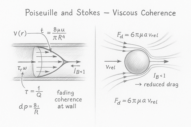
For an incompressible laminar flow in a circular pipe, energy conservation and shear balance yield:
$$ \Delta p = \frac{8\mu L Q}{\pi R^4}, \qquad \tau_w = \frac{4\mu \bar{v}}{R}. $$
Here:
Each streamline slides against its neighbour, creating a parabolic velocity profile:
$$ v(r) = v_{\mathrm{max}}\!\left(1 - \frac{r^2}{R^2}\right), \qquad v_{\mathrm{max}} = 2\bar{v}. $$
This is the signature of viscous coherence: the field distributes motion symmetrically through internal tension rather than turbulence or collisions.
In real systems, no surface is perfectly coherent.
A fraction of motion is lost through surface slip, microbubbles, roughness, or alignment failure.
We describe this with a viscous coherence index and a slip fraction :
$$ \Delta p = I_B(1 - s)\, \frac{8\mu L Q}{\pi R^4}. $$
Thus, viscosity becomes a measure not only of friction, but of how deeply the boundary geometry remembers the flow.
At low Reynolds number (), a sphere moving through a viscous fluid experiences a linear drag:
$$ F_d = 6\pi\mu a v_{\mathrm{rel}}. $$
This is Stokes’ law, where a is the sphere’s radius and is its velocity relative to the fluid.
Each layer of fluid wraps around the sphere, generating coherent shear.
The flow pattern is continuous and laminar — every particle of fluid communicates its motion through viscous tension.
With coherence correction:
$$ F_d = I_B(1 - s)\,6\pi\mu a v_{\mathrm{rel}}. $$
When coherence falls () or slip rises (), drag decreases.
The fluid “forgets” the boundary motion — partial slip appears, reducing energy coupling.
$$ F_d = (\rho_p - \rho)\, g\, \frac{4}{3}\pi a^3. $$
From Stokes’ law:
$$ v_{\mathrm{term}} = \frac{2}{9}\, \frac{(\rho_p - \rho)\, g\, a^2}{\mu}. $$
Adding coherence corrections:
$$ v_{\mathrm{term}} = \frac{1}{I_B(1 - s)}\, \frac{2}{9}\, \frac{(\rho_p - \rho)\, g\, a^2}{\mu}. $$
Lower coherence leads to faster settling — the boundary cannot sustain full viscous resistance.
This shows that viscous drag is not fixed but emergent — a property of how well the boundary remembers motion.
Poiseuille and Stokes describe two extremes of the same field geometry:
| Regime | Flow Geometry | Coherence Description |
|---|---|---|
|
Poiseuille
|
Layered channel
|
Coherence between |
|
Stokes
|
Curved enclosure
|
Coherence around
a closed surface |
|
Darcy (blend)
|
Transitional
|
Partial coherence,
early turbulence |
In all cases, the Reynolds number () represents the balance between coherence tension and inertial memory:
$$ \mathrm{Re} = \frac{\rho v D}{\mu}. $$
When is small, coherence dominates; when large, inertia carries memory forward faster than viscosity can realign it.
Turbulence is simply coherence breakdown — local curvature losing communication across boundaries.