
Chapter 17
Coulomb Flow and Charge Potential

Field and Energy Systems
Author: Mark Anthony Higgins
© Mark Anthony Higgins 11 October 2025
Revised Date: 23 February 2026
Audio Overview
Flow Algebra
flow "CoulombFlow_ChargePotential"

# ---------- STATES ----------
state:
  charge.q: float                     # charge magnitude (C)
  position.r: vec[float,3]            # field point position (m)
  source.r0: vec[float,3]             # source position (m)
  distance.R: float                   # |r - r0|
  potential.Φ: float                  # electrostatic potential (V)
  field.E: vec[float,3]               # electric field vector (V/m)
  permittivity.ε0: float              # permittivity of free space (F/m)
  boundary.integrity: float           # coherence of local curvature boundary (0..1)
  curvature.tension.Σ: float          # field curvature tension (J/m³)
  energy.density.ρE: float            # energy density (J/m³)
  flux.Jμ: vec[float,4]               # coherence flux (field current analogue)
  divergence.∇·E: float               # field divergence
  total.energy.U: float               # field energy (J)
  potential.surface.SΦ: surface       # equipotential surface geometry
  time.t: float

# ---------- PARAMETERS ----------
params:
  ε0: 8.854e-12
  k_e: 8.9875517923e9                # Coulomb constant (N·m²/C²)
  k_coh: float                       # curvature–coherence coupling constant
  dt: float

# ---------- INVARIANTS ----------
invariant:
  - potential.Φ = params.k_e * charge.q / distance.R
  - field.E = -∇Φ = (params.k_e * charge.q / distance.R²) * r̂
  - ∇·E = charge.q / (params.ε0)
  - energy.density.ρE = ½ params.ε0 |E|²
  - total.energy.U = ∫ ρE dV = ½ ∫ ρ Φ dV
  - boundary.integrity ≈ 1 for static isolated charge (stationary coherence)
  - coherence equation: ∂μ J^μ = 0  ↔ ∇·E = ρ/ε₀  (continuity of field coherence)
  - curvature.tension.Σ ∝ |E|²  (field curvature strength proportional to energy density)
  - like charges → boundary curvature repulsion; opposite charges → curvature complementarity (coherence closure)

# ---------- TRANSFORMS ----------
transform:

  initialise_field:
    do:
      charge.q = 1.0e-6              # 1 μC test charge
      source.r0 = [0,0,0]
      position.r = [1,0,0]
      distance.R = norm(position.r - source.r0)
      potential.Φ = params.k_e * charge.q / distance.R
      field.E = (params.k_e * charge.q / distance.R**2) * unit_vector(position.r - source.r0)
      boundary.integrity = 0.995
      time.t = 0

  compute_field:
    do:
      distance.R = norm(position.r - source.r0)
      field.E = (params.k_e * charge.q / distance.R**2) * unit_vector(position.r - source.r0)
      potential.Φ = params.k_e * charge.q / distance.R
      divergence.∇·E = charge.q / params.ε0

  compute_energy_density:
    do:
      energy.density.ρE = 0.5 * params.ε0 * dot(field.E, field.E)
      curvature.tension.Σ = params.k_coh * energy.density.ρE

  update_coherence_flux:
    do:
      flux.Jμ = [energy.density.ρE, field.E]  # energy density + directional flow
      boundary.integrity -= small_drift(energy.density.ρE)
      if boundary.integrity < 0.98:
        mark("radiative_coupling")

  check_superposition:
    do:
      # For multiple sources, linear superposition applies
      field.E_total = Σ_i (params.k_e * q_i * (r - r_i)) / |r - r_i|³
      potential.Φ_total = Σ_i (params.k_e * q_i / |r - r_i|)
      verify linearity(E_total, Φ_total)

  tick:
    do:
      time.t += params.dt

# ---------- MONITORS ----------
monitor:
  field_profile:
    observe: [distance.R, potential.Φ, |field.E|]
    report: "Potential ∝ 1/R, field ∝ 1/R² — verifies inverse-square curvature distribution."

  energy_balance:
    observe: [energy.density.ρE, total.energy.U]
    report: "Checks total field energy consistency with stored curvature tension."

  coherence_integrity:
    observe: [boundary.integrity]
    report: "Near 1 for static equilibrium; drift indicates dynamic coupling (radiation)."

# ---------- NOTES (coherence view) ----------
note:
  - Charge is the **geometric asymmetry** of curvature coherence — a region where boundary phase is shifted by 2πn + δΦ.
  - The Coulomb field is the **curvature tension gradient** caused by that phase offset; potential Φ measures curvature relaxation per unit charge.
  - The inverse-square law reflects how curvature distributes on a spherical boundary: flux through 4πr² constant.
  - In HST, ∇·E = ρ/ε₀ is identical to ∂μJμ = 0 — the continuity of coherence through the boundary.
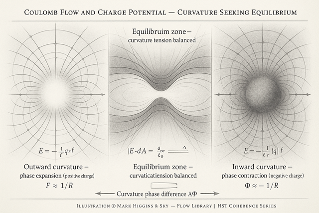
  - Positive charge = outward curvature (phase expansion); negative charge = inward curvature (phase contraction).
  - Electric potential energy represents **stored curvature tension** between boundaries.
  - Field superposition arises from additive coherence when curvature coupling is linear (no feedback).
  - Nonlinear regimes (strong fields) induce curvature feedback: field lines curve back upon themselves, producing self-energy corrections.
  - Thus, Coulomb flow is not “force through space” but **coherence realignment between boundaries** seeking equilibrium.

What this flow captures

CoulombFlow_ChargePotential reformulates classical electrostatics as a problem of boundary coherence and curvature tension, rather than forces acting through empty space.
In HST, a charge is not a material point but a localized phase imbalance — a region where the curvature of the coherence field diverges slightly from equilibrium.
The electric field is the gradient of that imbalance; the potential is the stored curvature tension between boundaries.

Thus, Coulomb’s law becomes a specific case of coherence redistribution:

\[ \partial_{\mu} J^{\mu}_{\mathrm{coh}} = 0 \;\Longleftrightarrow\; \nabla\!\cdot\!\mathbf{E} = \frac{\rho}{\varepsilon_{0}}\,. \]

The inverse-square field reflects how curvature coherence spreads over spherical boundaries to maintain constant flux.


Core intuition (HST view)
In the conventional view, a charge emits an electric field described by

\[ \mathbf{E} = \frac{1}{4\pi \varepsilon_{0}}\,\frac{q}{r^{2}}\,\hat{r}, \qquad \Phi = \frac{1}{4\pi \varepsilon_{0}}\,\frac{q}{r}\,. \]

In HST, this same relationship describes how boundary phase curvature relaxes through space: the field lines are coherence trajectories and the potential is their curvature energy density per unit phase.

  • Positive charge: outward curvature — phase expanding from centre.
  • Negative charge: inward curvature — phase collapsing toward centre.
  • Potential difference: difference in curvature tension between two boundaries.

When two charged boundaries interact, coherence flows from higher tension to lower — what we perceive as an electric force.


Mathematical structure

The electrostatic potential obeys Poisson’s equation:

\[ \nabla^{2}\Phi = -\frac{\rho}{\varepsilon_{0}}\,. \]

The field energy density is

\[ \rho_{E} = \tfrac{1}{2}\,\varepsilon_{0}\,|\mathbf{E}|^{2}\,. \]

Total stored energy:

\[ U = \tfrac{1}{2} \int \rho\,\Phi\, dV = \tfrac{1}{2}\,\varepsilon_{0} \int |\mathbf{E}|^{2}\, dV\,. \]

In HST, this stored energy is the curvature tension of the field:

\[ \Sigma \propto |\mathbf{E}|^{2}\,. \]

representing the amount of geometric distortion sustained by coherence at the boundary.
Electric field lines are curvature contours; equipotential surfaces are regions of constant coherence tension.


Interpreting charge through boundary coherence
Classical termHST interpretation
Charge \( q \)
Localised curvature asymmetry — net phase offset
Electric field \( \mathbf{E} \)
Gradient of coherence realignment
Potential \( \Phi \)
Scalar curvature tension energy per unit charge
Field energy \( q\,\mathbf{E} \)
Stored curvature tension density
Force 𝑞 𝐸
Restoring flow of coherence seeking boundary equilibrium
Superposition
Linear coherence overlay (additivity of phase gradients)

The field equations describe not action at a distance but the redistribution of curvature in a connected coherence fabric.


Boundary flux and conservation

The field flux through a closed surface,

\[ \oint_{S} \mathbf{E} \cdot d\mathbf{A} = \frac{q_{\mathrm{enc}}}{\varepsilon_{0}}\,. \]

is identical to the continuity of coherence current:

\[ \int_{V} \partial_{\mu} J^{\mu}_{\mathrm{coh}}\, dV = 0\,. \]

This ensures that curvature flow is divergence-free everywhere except where phase discontinuity (charge) exists.
When two charges approach, their curvature boundaries deform; the resulting overlap defines the potential energy of interaction.


Superposition and linearity
At low curvature tension, the field obeys perfect linearity:

\[ \Phi_{\mathrm{total}} = \sum_{i} \Phi_{i}, \qquad \mathbf{E}_{\mathrm{total}} = \sum_{i} \mathbf{E}_{i}\,. \]

Each charge contributes additively — coherence flows independently through the global field.
When field intensity rises, curvature feedback appears (nonlinear terms like
E
2
E
|\mathbf{E}|^2\mathbf{E}
 leading to self-interaction or dielectric breakdown — the geometric expression of nonlinearity.


Energy and coherence flow

The Poynting vector

\[ \mathbf{S} = \frac{1}{\mu_{0}}\,(\mathbf{E} \times \mathbf{B})\,. \]

in dynamic fields represents the directional flux of coherence energy.
In static Coulomb systems, that flux is zero on average — coherence tension is stored, not propagated.
A radiating charge is simply a boundary where coherence oscillates and releases stored curvature energy as electromagnetic waves.


Philosophical coherence
  • Charge is the geometry’s memory of imbalance — a residual phase displacement.
  • Potential is curvature tension — the “height” of coherence strain.
  • Field is not a substance but the path of coherence flow between boundaries.
  • Force is curvature’s way of restoring symmetry.

In the language of HST:

Charge is phase; potential is tension; field is geometry seeking equilibrium.


Significance

The Coulomb flow demonstrates that even the simplest field — electrostatics — obeys the same coherence law as gravity, fluid dynamics, or quantum phase.
Every “force” in physics is the movement of coherence tension toward equilibrium across a boundary.

When expressed this way, electromagnetism becomes not a separate interaction but a manifestation of curvature coherence in U(1) symmetry space — the harmonic of phase conservation predicted by Noether’s theorem.

At its heart, the Coulomb field is geometry remembering its imbalance, and potential is that memory’s stored tension.


In essence

Charge is not a thing but a curvature note in the field’s coherence song.
Potential is the pitch of that note — the strain of geometry awaiting release.
All fields, even the electric, are coherence seeking to heal their own asymmetry.


Kireth Research
38 Thorndale Croft, Wetwang, Driffield
East Riding of Yorkshire YO25 9XZ
Designed By