
Chapter 26
Finite-Time Engine Timed Strokes & Coherence Loss

Thermal and Entropic Flows
Author: Mark Anthony Higgins
© Mark Anthony Higgins 11 October 2025
Revised Date: 23 February 2026
Audio Overview
Flow Algebra
flow "Finite-Time Engine — Timed Strokes & Coherence Loss" v1.1


# ---------- IO (CSV export; safe for Excel) ----------
io.write:
  format: csv
  encoding: utf-8-sig
  filename: "finite_time_engine_results_${run_id}.csv"
  schema:
    - cycle:int
    - t_end:float
    - Q_in:float
    - Q_out:float
    - W_out:float
    - eta:float
    - Sigma:float
    - T_hot:float
    - T_cold:float
    - G_hot:float
    - G_cold:float
    - IB_hot:float
    - IB_cold:float
    - tau_total:float
    - scene:str?

# ---------- PARAMETERS ----------
params:
  units: "SI"
  # Reservoir temps and exchanger conductances
  T_hot:   positive
  T_cold:  positive
  G_hot:   positive        # [W/K]
  G_cold:  positive        # [W/K]
  # Working fluid (ideal-gas guide)
  gamma:   positive        # Cp/Cv (e.g., 1.4)
  R:       positive = 8.314462618
  # Boundary coherence indices (1=reversible)
  IB_hot:  0.0..1.0
  IB_cold: 0.0..1.0
  # Stroke timings
  cycle:
    tau_hot:      positive # s
    tau_expand:   positive # s
    tau_cold:     positive # s
    tau_compress: positive # s
  sign_convention:
    heat_in_positive: true   # into WF
    work_out_positive: true  # done by WF

# ---------- STATE ----------
state WorkingFluid:
  U: real
  S: real
  T: positive
  p: positive
  V: positive
  n: positive              # moles (closed WF)

state Ports:
  Qdot_hot:  real          # + from hot reservoir
  Qdot_cold: real          # + from cold reservoir (usually negative)
  Wdot_out:  real          # mechanical power out

state StrokeTimer:
  t: real = 0.0
  phase ∈ {hot_iso, expand_ad, cold_iso, compress_ad}

state CycleTotals (reset each cycle):
  Q_in:   real = 0
  Q_out:  real = 0
  W_out:  real = 0
  Sigma:  real = 0

state Results:
  run_id: str  = now_timestamp_compact
  cycle_no: int = 0
  t_prev:  real = 0

# ---------- CORE LAWS ----------
invariants:
  # First law (instantaneous)
  ddt(WorkingFluid.U) = Ports.Qdot_hot + Ports.Qdot_cold - Ports.Wdot_out
  # Second law
  ddt(WorkingFluid.S) = Ports.Qdot_hot/WorkingFluid.T + Ports.Qdot_cold/WorkingFluid.T + sigma
  sigma >= 0

  # Physical positivity
  WorkingFluid.T > 0; WorkingFluid.V > 0; WorkingFluid.p > 0

# ---------- SCHEDULER ----------
transforms scheduler:
  total_tau = params.cycle.tau_hot + params.cycle.tau_expand + params.cycle.tau_cold + params.cycle.tau_compress
  if 0 <= StrokeTimer.t < params.cycle.tau_hot:
    StrokeTimer.phase = hot_iso
  if params.cycle.tau_hot <= StrokeTimer.t < params.cycle.tau_hot + params.cycle.tau_expand:
    StrokeTimer.phase = expand_ad
  if params.cycle.tau_hot + params.cycle.tau_expand <= StrokeTimer.t < params.cycle.tau_hot + params.cycle.tau_expand + params.cycle.tau_cold:
    StrokeTimer.phase = cold_iso
  if params.cycle.tau_hot + params.cycle.tau_expand + params.cycle.tau_cold <= StrokeTimer.t < total_tau:
    StrokeTimer.phase = compress_ad
  if StrokeTimer.t >= total_tau:
    StrokeTimer.t = 0

# ---------- IDEAL-GAS GUIDE ----------
transforms ideal_gas_guide:
  WorkingFluid.p = (WorkingFluid.n * params.R * WorkingFluid.T) / WorkingFluid.V

# ---------- STROKE MODELS ----------
transforms hot_isothermal (when StrokeTimer.phase == hot_iso):
  Ports.Qdot_hot = params.G_hot * (params.T_hot - WorkingFluid.T)
  Ports.Wdot_out = WorkingFluid.p * ddt(WorkingFluid.V)
  # Entropy production from finite ΔT and exchanger loss via IB_hot
  sigma += Ports.Qdot_hot * (1/WorkingFluid.T - 1/params.T_hot)
  phi_hot >= (1 - params.IB_hot) * max(Ports.Qdot_hot, 0)
  sigma += phi_hot / max(WorkingFluid.T, 1e-12)

transforms adiabatic_expand (when StrokeTimer.phase == expand_ad):
  Ports.Qdot_hot  = 0
  Ports.Qdot_cold = 0
  Ports.Wdot_out  = WorkingFluid.p * ddt(WorkingFluid.V) - phi_mech
  phi_mech >= 0
  sigma += phi_mech / WorkingFluid.T
  # Monitor (guide): T*V^{γ-1} ≈ const (not enforced)

transforms cold_isothermal (when StrokeTimer.phase == cold_iso):
  Ports.Qdot_cold = params.G_cold * (params.T_cold - WorkingFluid.T)   # typically negative
  Ports.Wdot_out  = WorkingFluid.p * ddt(WorkingFluid.V)
  sigma += Ports.Qdot_cold * (1/WorkingFluid.T - 1/params.T_cold)
  phi_cold >= (1 - params.IB_cold) * max(-Ports.Qdot_cold, 0)
  sigma += phi_cold / max(WorkingFluid.T, 1e-12)

transforms adiabatic_compress (when StrokeTimer.phase == compress_ad):
  Ports.Qdot_hot  = 0
  Ports.Qdot_cold = 0
  Ports.Wdot_out  = WorkingFluid.p * ddt(WorkingFluid.V) - phi_mech
  phi_mech >= 0
  sigma += phi_mech / WorkingFluid.T

# ---------- SIMPLE VOLUME PROGRAM (piecewise-linear per stroke) ----------
# Define targets V1 -> V2 -> V3 -> V2 -> V1 across the four phases.
transforms volume_program:
  V1 = V_min; V2 = V_mid; V3 = V_max
  if StrokeTimer.phase == hot_iso:
    dVdt = (V2 - V1) / params.cycle.tau_hot
  if StrokeTimer.phase == expand_ad:
    dVdt = (V3 - V2) / params.cycle.tau_expand
  if StrokeTimer.phase == cold_iso:
    dVdt = (V2 - V3) / params.cycle.tau_cold
  if StrokeTimer.phase == compress_ad:
    dVdt = (V1 - V2) / params.cycle.tau_compress
  ddt(WorkingFluid.V) = dVdt

# ---------- ACCUMULATORS ----------
transforms accumulate:
  if StrokeTimer.phase == hot_iso:
    CycleTotals.Q_in  += Ports.Qdot_hot  * dt
  if StrokeTimer.phase == cold_iso:
    CycleTotals.Q_out += (-Ports.Qdot_cold) * dt
  CycleTotals.W_out   += Ports.Wdot_out * dt
  CycleTotals.Sigma   += sigma * dt

# ---------- CSV LOGGER ----------
transforms detect_cycle_boundary:
  if StrokeTimer.t < Results.t_prev:
    Results.cycle_no += 1
    call finalize_and_flush_cycle
  Results.t_prev = StrokeTimer.t

transforms finalize_and_flush_cycle:
  eta_cycle = CycleTotals.W_out / max(CycleTotals.Q_in, 1e-12)
  tau_total = params.cycle.tau_hot + params.cycle.tau_expand + params.cycle.tau_cold + params.cycle.tau_compress
  io.write.append:
    cycle:     Results.cycle_no
    t_end:     StrokeTimer.t + tau_total
    Q_in:      CycleTotals.Q_in
    Q_out:     CycleTotals.Q_out
    W_out:     CycleTotals.W_out
    eta:       eta_cycle
    Sigma:     CycleTotals.Sigma
    T_hot:     params.T_hot
    T_cold:    params.T_cold
    G_hot:     params.G_hot
    G_cold:    params.G_cold
    IB_hot:    params.IB_hot
    IB_cold:   params.IB_cold
    tau_total: tau_total
    scene:     active_scene_label?
  # reset
  CycleTotals.Q_in  = 0
  CycleTotals.Q_out = 0
  CycleTotals.W_out = 0
  CycleTotals.Sigma = 0

# ---------- MONITORS ----------
monitors:
  efficiency_bound:
    eta_inst = CycleTotals.W_out / max(CycleTotals.Q_in, 1e-12)
    eta_carnot = 1 - params.T_cold/params.T_hot
    assert eta_inst <= eta_carnot + 1e-9
  positivity:
    assert sigma >= 0
    assert WorkingFluid.T > 0 && WorkingFluid.V > 0
  adiabatic_guide_check:
    # soft check (no failure): log deviation from T*V^{γ-1}
    C_ad = WorkingFluid.T * pow(WorkingFluid.V, params.gamma - 1)
    log.debug = "Adiabatic guide C = ${round(C_ad,6)}"

# ---------- DEFAULT SCENE (drop-in demo) ----------
scenes:
  starter_demo_ideal_gas:
    active_scene_label: "starter_demo_ideal_gas"
    given params:
      T_hot:  700.0
      T_cold: 300.0
      G_hot:  40.0
      G_cold: 40.0
      gamma:  1.4
      IB_hot: 0.95
      IB_cold:0.95
      cycle:
        tau_hot:      0.50
        tau_expand:   0.25
        tau_cold:     0.50
        tau_compress: 0.25
    given WorkingFluid:
      n: 0.10
      T: 450.0
      V: 1.00e-3
    given:
      V_min: 1.00e-3
      V_mid: 1.35e-3
      V_max: 1.80e-3
    enable:
      - scheduler
      - ideal_gas_guide
      - volume_program
      - hot_isothermal
      - adiabatic_expand
      - cold_isothermal
      - adiabatic_compress
      - accumulate
      - detect_cycle_boundary
Overview

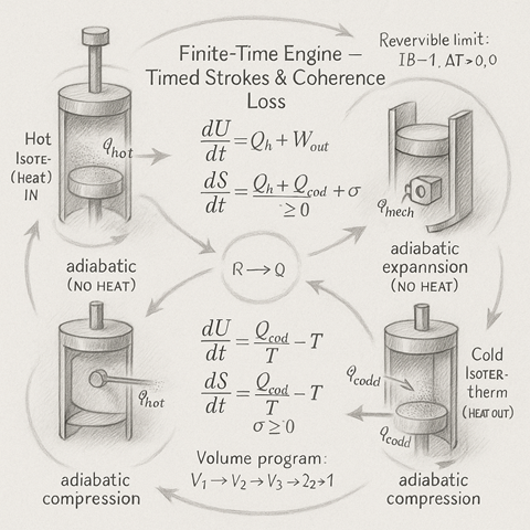
This flow turns the reversible symmetry of Work and Heat — Reciprocal Flows into a time-sequenced engine with real-world losses. Instead of assuming perfect, quasi-static steps, it models a four-stroke cycle with explicit contact times, finite thermal conductances, and coherence-dependent dissipation. You can watch efficiency rise as gradients shrink and boundary coherence improves — and fall when strokes are rushed or interfaces scatter energy.


Core Idea

At each instant the engine obeys:

$$ \frac{dU}{dt} = \dot{Q}_{\mathrm{hot}} + \dot{Q}_{\mathrm{cold}} - \dot{W}_{\mathrm{out}}, \qquad \frac{dS}{dt} = \frac{\dot{Q}_{\mathrm{hot}}}{T} + \frac{\dot{Q}_{\mathrm{cold}}}{T} + \sigma, \qquad \sigma \ge 0. $$

Loss enters via entropy production σ\sigma, sourced by finite temperature gaps, frictional terms, and imperfect boundaries. When coherence is high and gradients are small, σ→0\sigma\to 0 and the cycle approaches the reversible ideal.

Timed Strokes (structure)
  • 1. Hot isothermal (heat in): finite conductance \( G_{\mathrm{hot}} \) drives \(\dot{Q}_{\mathrm{hot}} = G_{\mathrm{hot}} (T_{\mathrm{hot}} - T)\). Work is produced as the volume expands, and entropy production includes a term proportional to the finite temperature difference \( \Delta T \).
  • 2. Adiabatic expand: no heat exchange (\(\dot{Q} = 0\)); mechanical output is reduced by a frictional loss \(\phi_{\mathrm{mech}}\).
  • 3. Cold isothermal (heat out): \(\dot{Q}_{\mathrm{cold}} = G_{\mathrm{cold}} (T_{\mathrm{cold}} - T)\) (typically negative). Compression work is done on the working fluid, and the finite temperature difference \( \Delta T \) contributes to entropy production \( \sigma \).
  • 4. Adiabatic compress: the system returns to its starting state; no heat exchange (\(\dot{Q} = 0\)), and frictional effects again contribute to entropy production \(\sigma\).

A simple piecewise-linear \(V(t)\) program sets each stroke’s expansion/compression rate, so you can directly explore the trade-off between cycle time and reversibility.

Boundary Coherence (IB)

<Each exchanger carries a coherence index \( I_B \in [0,\,1] \).

  • \( I_B = 1:\) near-ideal coupling; minimal scattering or radiation; entropy production \( \sigma \) is small.
  • \( I_B < 1:\) partial coherence; additional dissipation \( \phi \) raises entropy production \( \sigma \). This turns “loss” into a measurable, tunable parameter — linking material interfaces directly to thermodynamic performance.
Performance & Bounds

Per-cycle metrics are logged to CSV: \( Q_{\mathrm{in}}, Q_{\mathrm{out}}, W, \eta, \Sigma. \) Efficiency is monitored against the Carnot limit \( \eta_{\mathrm{Carnot}} = 1 - \tfrac{T_{\mathrm{cold}}}{T_{\mathrm{hot}}}. \) As contact times increase and \( I_B \to 1, \) the efficiency \( \eta \) approaches this bound; pushing speed or lowering \( I_B \) increases total entropy generation \( \Sigma \) and reduces \( \eta. \)


What to vary (experiments)
  • Timing: lengthen \( \tau_{\mathrm{hot}} \) and \( \tau_{\mathrm{cold}} \) to reduce the temperature difference \( \Delta T \) and observe an increase in efficiency \( \eta \!\uparrow\! \).
  • Conductance: increase \( G_{\mathrm{hot}} \) and \( G_{\mathrm{cold}} \) to improve heat transfer at fixed cycle time.
  • Coherence: raise \( I_{B_{\mathrm{hot}}} \) and \( I_{B_{\mathrm{cold}}} \) to reduce boundary losses and approach the reversible limit.
  • Stroke geometry: widen \( V_{\min} \!\to\! V_{\max} \) for larger work output — but note increased sensitivity to frictional losses \( \phi_{\mathrm{mech}} \).
  • Speed–reversibility curve: plot efficiency \( \eta \) versus total cycle time to reveal the classic finite-time trade-off between speed and reversibility.
How this extends the Reciprocity Flow

The Work & Heat flow defines the local symmetry (reciprocal channels, σ→0\sigma\to 0 in the ideal).
This engine introduces time and interface reality — showing exactly how reciprocity breaks when you run fast or couple imperfectly, and how coherence can be engineered back in.


Implementation notes
  • The flow includes an ideal-gas guide (for \( pV = nRT \)) and optional adiabatic checks.
  • A starter scene is provided; enable the scheduler, stroke transforms, and CSV logger to run.
  • Results are Excel-safe (UTF-8 with BOM), ready for plotting efficiency \( \eta \) and entropy generation \( \Sigma \) across cycles.

Engineer’s Checklist — Running the Finite-Time Engine Flow

Use this checklist to tune your engine parameters and observe how coherence, timing, and transfer geometry shape real performance.

⚙️ 1. Thermal Setup
ParameterTypical RangeNotes
T_hot

500 – 900 K

Set by hot reservoir or heater model.

T_cold
250 – 350 K
Ambient or coolant temperature.
G_hot, G_cold
10 – 100 W/K
Thermal conductance;
higher values = faster equalisation
but heavier hardware.

**Tip:** keep \( G_{\mathrm{hot}} \approx G_{\mathrm{cold}} \) for symmetric balance, unless intentionally testing asymmetric cycles.


🧭 2. Stroke Timing
PhaseSymbolTypical Duration

Hot isothermal

τh

0.3 – 1.0 s

Adiabatic expand
τₑ
0.1 – 0.5 s
Cold isothermal
τ_c
0.3 – 1.0 s
Adiabatic compress
τₐ
0.1 – 0.5 s
Guideline:
  • Slower cycles (long τ): smaller ΔT, less σ, higher η.
  • Faster cycles: greater ΔT, larger σ, lower η — test coherence resilience.

🔁 3. Boundary Coherence (IB)
IB valueBehaviourInterpretation
1.00
Reversible limit
Perfectly matched boundary, σ ≈ 0.
0.85
Mild loss
Realistic metallic contact.
0.60
Significant loss
Surface scattering, poor polish.
< 0.4
Chaotic
Thermal leakage dominates; engine mostly dissipative.
One
One
two

Rule: η roughly scales with IB² near the reversible regime


⚖️ 4. Geometry & Working Fluid
ParameterSymbolGuidance
Moles of gas
n
0.05 – 0.2 mol for lab scale
Volume ratio

Vmax / Vmin

1.5 – 2.0 typical
\(\gamma = \dfrac{C_p}{C_v}\)

1.4 (air), 1.67 (monoatomic)

Adjust for fluid type

Tip: Use small volume ratios for sensitivity studies; large ratios amplify deviations and highlight coherence effects


🔍 5. Observables
QuantitySymbolInterpretation
Efficiency
η = W_out / Q_in
Approaches 1 – T₍c₎/T₍h₎ when IB→1 and σ→0.
Entropy generation
Σ
Measures coherence loss per cycle.
ΔQ = Q_in – Q_out – W_out
Energy balance check (≈ 0).
η / η₍Carnot₎
Coherence ratio of operation.
Plot idea:

η vs. cycle time or IB to show the speed–reversibility curve — the visual fingerprint of every finite-time system.


💡 6. Practical Insight
  • Every boundary is a memory: the closer its microstructure matches the working field, the smaller the loss.
  • Efficiency is not just thermal — it’s a measure of coherence retention per cycle.
  • Slow, coherent engines trace elegant loops; rushed, incoherent ones blur into heat.

Kireth Research
38 Thorndale Croft, Wetwang, Driffield
East Riding of Yorkshire YO25 9XZ
Designed By