Chapter 23
Poynting Vector and Energy Transfer
Field and Energy Systems
Author: Mark Anthony Higgins
© Mark Anthony Higgins 11 October 2025
Revised Date: 23 February 2026
flow "PoyntingVector_EnergyTransfer"
# ---------- STATES ----------
state:
# field values on region V with boundary Γ
field.E: vec[float,3] # electric field (V/m)
field.B: vec[float,3] # magnetic field (T)
field.grad: tensor # ∇E, ∇B (optional for stress calc)
# material properties (effective, possibly piecewise)
material.εr: float # relative permittivity
material.μr: float # relative permeability
material.σ: float # conductivity (S/m)
# sources
source.ρ: float # charge density (C/m^3)
source.J: vec[float,3] # current density (A/m^2)
# energy & flux bookkeeping
energy.u: float # field energy density (J/m^3)
poynting.S: vec[float,3] # Poynting vector (W/m^2)
flux.Φ_SΓ: float # ∮_Γ S·n dA (W) outward flux
work.power_on_charges: float # ∫_V J·E dV (W)
loss.ohmic: float # ∫_V σ|E|^2 dV (W) if σ>0
stress.T: tensor # Maxwell stress tensor on Γ
pressure.boundary: float # n·T·n on Γ (Pa)
# region geometry & integration handles
region.V: volume
region.Γ: surface
normal.n: fn(vec3)->vec3 # outward unit normal on Γ
# boundary coherence bookkeeping
boundary.type: "free"|"conductor"|"dielectric"
boundary.integrity.IB: float # 0..1 coherence integrity
# running integrals
energy.U_total: float # ∫_V u dV (J)
energy.U_prev: float # previous step U_total
balance.residual: float # ΔU + Φ_SΓ + ∫V J·E dV (should ≈0)
time.t: float
# ---------- PARAMETERS ----------
params:
ε0: 8.8541878128e-12
μ0: 1.25663706212e-6 # 4π×10^-7 H/m
dt: float
integrate.surface_resolution: int
integrate.volume_resolution: int
use.medium_form: bool # if true, use ε=ε0εr, μ=μ0μr
log.stress: bool
log.flux_field: bool
# ---------- INVARIANTS ----------
invariant:
- medium.coeffs:
ε = params.ε0 * (material.εr if use.medium_form else 1.0)
μ = params.μ0 * (material.μr if use.medium_form else 1.0)
- energy_density:
energy.u = 0.5 * ( ε * |field.E|^2 + (1/μ) * |field.B|^2 )
- poynting_vector:
poynting.S = (1/μ) * cross(field.E, field.B)
- poynting_theorem_local:
∂t(energy.u) + div(poynting.S) = - dot(source.J, field.E)
- ohmic_heating:
loss.joule_density = material.σ * |field.E|^2
- maxwell_stress_tensor:
stress.T = ε * ( outer(field.E, field.E) - 0.5*|field.E|^2 * I )
+ (1/μ) * ( outer(field.B, field.B) - 0.5*|field.B|^2 * I )
- boundary_conditions:
conductor: E_tan = 0 on Γ, B_norm = 0 on Γ
dielectric: ε1 E_norm(1) = ε2 E_norm(2), (B/μ)_tan continuous
- coherence_continuity (global V):
d/dt ∫_V u dV + ∮_Γ S·n dA = - ∫_V J·E dV
# ---------- TRANSFORMS ----------
transform:
sample_fields:
do:
field.E = E_field(region.V, time.t)
field.B = B_field(region.V, time.t)
field.grad = gradients(field.E, field.B) # optional/approx
compute_energy_and_flux:
do:
energy.u = 0.5 * ( ε * |field.E|^2 + (1/μ) * |field.B|^2 )
poynting.S = (1/μ) * cross(field.E, field.B)
energy.U_prev = energy.U_total
energy.U_total = volume_integral(region.V, energy.u, integrate.volume_resolution)
flux.Φ_SΓ = surface_integral(region.Γ, dot(poynting.S, normal.n(x)), integrate.surface_resolution)
compute_work_terms:
do:
work.power_on_charges = volume_integral(region.V, dot(source.J, field.E), integrate.volume_resolution)
loss.ohmic = volume_integral(region.V, material.σ * |field.E|^2, integrate.volume_resolution)
boundary_reaction:
pre:
require boundary.type != null
do:
if params.log.stress:
stress.T = maxwell_stress(field.E, field.B, ε, μ)
pressure.boundary = surface_integral(region.Γ, quadform(normal.n(x), stress.T), integrate.surface_resolution)
# simple integrity bookkeeping: surge in boundary pressure reduces IB
boundary.integrity.IB = clamp(boundary.integrity.IB - surge_metric(pressure.boundary), 0, 1)
check_energy_balance:
do:
ΔU = (energy.U_total - energy.U_prev) / params.dt
balance.residual = ΔU + flux.Φ_SΓ/1.0 + work.power_on_charges
# Note: work.power_on_charges > 0 means energy is leaving the field and doing work on charges
tick:
do:
time.t += params.dt
# ---------- MONITORS ----------
monitor:
energy_conservation:
observe: [energy.U_total, flux.Φ_SΓ, work.power_on_charges, balance.residual]
report: "Checks global Poynting balance: dU/dt + ∮S·n = -∫J·E (residual→0)."
flux_map:
observe: [poynting.S]
report: "Vector field of energy flow; outward flux through Γ is positive."
ohmic_heating:
observe: [loss.ohmic]
report: "Joule loss ∫σ|E|^2 dV; equals work on charges in simple conductors."
boundary_pressure:
observe: [pressure.boundary, boundary.integrity.IB]
report: "Normal stress n·T·n on Γ and coherence integrity update."
field_energy_density:
observe: [energy.u]
report: "Tracks spatial distribution of ½(εE² + B²/μ)."
# ---------- NOTES (coherence view) ----------
note:
- **Meaning of S = (1/μ) E×B**: local, directed flow of coherence energy. Where S points, energy moves.
- **Field energy** u = ½(εE² + B²/μ) stores curvature tension (E) and curvature rotation (B).
- **Poynting theorem** is the energy continuity law: any drop in field energy within V is explained exactly by
(i) energy leaving through the boundary (∮ S·n dA) and
(ii) energy delivered to matter (∫ J·E dV).
- In **good conductors**, J≈σE ⇒ ∫J·E ≈ ∫σE² = ohmic heating; field energy becomes thermal/mechanical energy.
- **Maxwell stress** translates field momentum into mechanical pressure/traction on boundaries; it is the momentum analogue of S.
- **Coherence perspective (HST)**:
• E is phase-gradient tension; B is rotational coherence.
• S is phase-transport: coherence flowing to restore balance.
• Boundaries do not “eat” energy; they **redirect** it—into motion, heat, or transmitted fields—so that ∂μJ_coh^μ = 0 holds globally.
- Practical cues:
• Standing waves: U_total oscillates while time-averaged Φ_SΓ≈0.
• Waveguides: S hugs the guide; boundary pressure tracks guide loading.
• Dielectric stacks: discontinuities in ε, μ bend S; partial reflection/transmission split energy flow.
# ---------- WHAT THIS FLOW CAPTURES ----------
doc:
summary: >
PoyntingVector_EnergyTransfer provides a region-level energy audit for
electromagnetism. It computes field energy density, energy flux, work on
charges, and boundary stresses, and verifies the Poynting theorem as a
conservation statement. In the coherence framing, it shows how curvature
energy moves (S), stores (u), and couples to matter (J·E) without loss of
total coherence—only redistribution across field, boundary, and material.
Interpretation and Coherence View
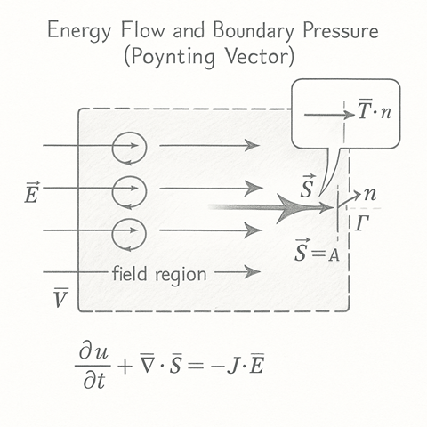
The Poynting vector
\[ \mathbf{S} = \frac{1}{\mu} \, \mathbf{E} \times \mathbf{B} \]
represents the flow of electromagnetic energy through space — the visible current of coherence itself.
Where E is the local curvature tension (phase gradient) and B is the rotational coherence (twist), their cross-product describes how coherence moves: tension redirected by rotation, energy transported by symmetry.
The field’s stored energy per unit volume is
\[ u = \tfrac{1}{2} \left( \varepsilon E^{2} + \frac{B^{2}}{\mu} \right) \]
and the continuity law (Poynting theorem) unites storage, flow, and transfer:
\[ \frac{\partial u}{\partial t} + \nabla \!\cdot\! \mathbf{S} = -\,\mathbf{J} \!\cdot\! \mathbf{E} \]
It states that any change in field energy within a region comes from two sources only:
Nothing is lost. The fields, particles, and boundaries form one continuous accounting system — a perfect coherence loop.
At a boundary, the Poynting vector bends, reflects, or transmits according to the medium’s impedance:
conductors return energy (mirror-like), dielectrics share it, and absorptive materials convert it into lattice motion or heat.
Yet even this “loss” is only translation — coherence reshaped into another form.
The Maxwell stress tensor
\[ T_{ij} = \varepsilon \!\left(E_{i}E_{j} - \tfrac{1}{2}E^{2}\delta_{ij}\right) + \frac{1}{\mu} \!\left(B_{i}B_{j} - \tfrac{1}{2}B^{2}\delta_{ij}\right) \]
extends this to momentum: it tells how energy flow exerts pressure and traction on surfaces.
The quantity n·T·n gives the normal stress — the mechanical touch of the field upon matter.
This is how light pushes sails, and why electromagnetic waves can sculpt matter at microscopic scales.
From the perspective of Holographic Space-Time,
the Poynting vector is coherence in motion — the re-balancing of curvature tension as the field exchanges structure with its surroundings.
Energy density u is the local curvature reservoir;
J·E is the translation of that curvature into motion or heat;
and the stress tensor T is how curvature transmits momentum between boundaries.
At perfect coherence ( ∂μ J_coh^μ = 0 ),
every watt leaving one domain enters another: light absorbed becomes warmth, tension released becomes motion, and reflection becomes organised redirection.
No part of the system is ever isolated — all boundaries are translators of coherence.
The Poynting vector is not merely a mathematical construct — it is geometry in transit.
It shows where the universe is currently remembering itself, transferring curvature from one form to another.
Energy is never lost — only translated.
Every photon, reflection, and field pressure is the same act repeated in different languages:
geometry preserving its own continuity.
Energy Density
\( u = \tfrac{1}{2}(\varepsilon |\mathbf{E}|^{2} + |\mathbf{B}|^{2}/\mu) \)
Poynting Vector
\( \mathbf{S} = (1/\mu)\,\mathbf{E} \times \mathbf{B} \)
Local Continuity Law
\( \dfrac{\partial u}{\partial t} + \nabla \!\cdot\! \mathbf{S} = -\,\mathbf{J}\!\cdot\!\mathbf{E} \)
Integral Form
\( \dfrac{d}{dt}\!\int_{V} u\,dV + \!\oint_{\Gamma}\! \mathbf{S}\!\cdot\!\mathbf{n}\,dA = -\!\int_{V}\! \mathbf{J}\!\cdot\!\mathbf{E}\,dV \)
Maxwell Stress Tensor
\( T_{ij} = \varepsilon(E_iE_j - \tfrac{1}{2}E^{2}\delta_{ij}) + \tfrac{1}{\mu}(B_iB_j - \tfrac{1}{2}B^{2}\delta_{ij}) \)
Boundary Pressure
\( P_{\text{boundary}} = \mathbf{n}\!\cdot\!\mathbf{T}\!\cdot\!\mathbf{n} \)
Coherence Form (HST)
\( \partial_{\mu}J_{\text{coh}}^{\mu}=0 \;\;\Longleftrightarrow\;\; \text{energy–momentum continuity across field, matter, and boundary.} \)
In the language of coherence, the Poynting vector is light remembering where to go.