flow "Finite-Time Engine — Timed Strokes & Coherence Loss" v1.0
authors: ["Mark Higins","Sky AI"]
locale: "en-GB"

# ---------- PARAMETERS ----------
params:
  units: "SI"
  T_hot: positive
  T_cold: positive
  G_hot: positive        # hot-side thermal conductance [W/K]
  G_cold: positive       # cold-side thermal conductance [W/K]
  gamma: positive        # heat capacity ratio (ideal gas scene)
  R: positive = 8.314462618
  IB_hot: 0.0..1.0       # coherence index on hot exchanger
  IB_cold: 0.0..1.0
  cycle:
    tau_hot:  positive   # contact time with hot reservoir
    tau_expand: positive # adiabatic/finite-time expand
    tau_cold:  positive
    tau_compress: positive
  sign_convention:
    heat_in_positive: true
    work_out_positive: true

# ---------- STATE ----------
state WorkingFluid:
  U: real
  S: real
  T: positive
  p: real
  V: positive
  n: positive            # moles (closed WF)

state Ports:
  Qdot_hot:  real        # + into WF from hot
  Qdot_cold: real        # + into WF from cold (usually negative)
  Wdot_out:  real

# ---------- STROKE SCHEDULER ----------
state StrokeTimer:
  t: real
  phase ∈ {hot_iso, expand_ad, cold_iso, compress_ad}

transforms:
  scheduler:
    if 0        <= StrokeTimer.t < params.cycle.tau_hot:        StrokeTimer.phase = hot_iso
    if tau_hot  <= t < tau_hot+tau_expand:                      StrokeTimer.phase = expand_ad
    if tau_hot+tau_expand <= t < tau_hot+tau_expand+tau_cold:   StrokeTimer.phase = cold_iso
    if tau_hot+tau_expand+tau_cold <= t < tau_hot+tau_expand+tau_cold+tau_compress:
                                                               StrokeTimer.phase = compress_ad
    if t ≥ total_tau: t = 0   # loop cycle
  total_tau = params.cycle.tau_hot + params.cycle.tau_expand + params.cycle.tau_cold + params.cycle.tau_compress

# ---------- LAW CORE ----------
invariants:
  # First law (instantaneous):
  ddt(WorkingFluid.U) = Ports.Qdot_hot + Ports.Qdot_cold - Ports.Wdot_out
  # Second law:
  ddt(WorkingFluid.S) = Ports.Qdot_hot/WorkingFluid.T + Ports.Qdot_cold/WorkingFluid.T + sigma
  sigma >= 0
  WorkingFluid.T > 0; WorkingFluid.V > 0

# ---------- STROKE MODELS ----------
transforms hot_isothermal (when StrokeTimer.phase == hot_iso):
  # Finite-time isothermal with heat leak/dissipation via IB_hot
  Ports.Qdot_hot = params.G_hot * (params.T_hot - WorkingFluid.T)
  # Ideal isothermal work element (e.g., ideal gas): Ẇ ≈ p·V̇ ; pV = nRT
  Ports.Wdot_out = WorkingFluid.p * ddt(WorkingFluid.V)
  # Entropy production from finite ΔT:
  sigma += Ports.Qdot_hot * (1/WorkingFluid.T - 1/params.T_hot)
  # Coherence loss mapping:
  phi_hot >= (1 - params.IB_hot) * max(Ports.Qdot_hot, 0)
  sigma += phi_hot / max(WorkingFluid.T, 1e-12)

transforms adiabatic_expand (when StrokeTimer.phase == expand_ad):
  Ports.Qdot_hot  = 0
  Ports.Qdot_cold = 0
  # Finite-time adiabatic with frictional dissipation:
  Ports.Wdot_out = WorkingFluid.p * ddt(WorkingFluid.V) - phi_mech
  phi_mech >= 0
  sigma += phi_mech / WorkingFluid.T
  # Ideal-gas guide (optional): T·V^{γ-1} ≈ const (monitor only)

transforms cold_isothermal (when StrokeTimer.phase == cold_iso):
  Ports.Qdot_cold = params.G_cold * (params.T_cold - WorkingFluid.T)  # usually negative
  Ports.Wdot_out  = WorkingFluid.p * ddt(WorkingFluid.V)
  sigma += Ports.Qdot_cold * (1/WorkingFluid.T - 1/params.T_cold)
  phi_cold >= (1 - params.IB_cold) * max(-Ports.Qdot_cold, 0)  # loss on rejection
  sigma += phi_cold / max(WorkingFluid.T, 1e-12)

transforms adiabatic_compress (when StrokeTimer.phase == compress_ad):
  Ports.Qdot_hot  = 0
  Ports.Qdot_cold = 0
  Ports.Wdot_out  = WorkingFluid.p * ddt(WorkingFluid.V) - phi_mech
  phi_mech >= 0
  sigma += phi_mech / WorkingFluid.T

# ---------- CYCLE ACCUMULATORS ----------
state CycleTotals (reset each cycle):
  Q_in:   real
  Q_out:  real
  W_out:  real
  Sigma:  real

transforms accumulate:
  if StrokeTimer.phase == hot_iso:
    CycleTotals.Q_in  += Ports.Qdot_hot * dt
  if StrokeTimer.phase == cold_iso:
    CycleTotals.Q_out += (-Ports.Qdot_cold) * dt   # magnitude rejected
  CycleTotals.W_out   += Ports.Wdot_out * dt
  CycleTotals.Sigma   += sigma * dt

# ---------- PERFORMANCE ----------
monitors:
  efficiency:
    eta = CycleTotals.W_out / max(CycleTotals.Q_in, 1e-12)
  carnot_bound:
    eta_carnot = 1 - params.T_cold / params.T_hot
    assert eta <= eta_carnot + 1e-9

  reversibility_indicator:
    if params.IB_hot ≈ 1 and params.IB_cold ≈ 1 and CycleTotals.Sigma ≈ 0:
      assert abs(eta - eta_carnot) <= 1e-6

  positivity:
    assert CycleTotals.Sigma >= 0
SIMPLE VOLUME PROGRAM
# ---------- SIMPLE VOLUME PROGRAM (piecewise-linear per stroke) ----------
transforms volume_program:
  # Define linear dV/dt for each phase to hit target endpoints exactly.
  # Hot isothermal:   V1 -> V2 (expand)
  # Adiabatic expand: V2 -> V3 (expand)
  # Cold isothermal:  V3 -> V2 (compress)
  # Adiabatic comp.:  V2 -> V1 (compress)
  V1 = V_min
  V2 = V_mid
  V3 = V_max

  if StrokeTimer.phase == hot_iso:
    dVdt = (V2 - V1) / params.cycle.tau_hot
  if StrokeTimer.phase == expand_ad:
    dVdt = (V3 - V2) / params.cycle.tau_expand
  if StrokeTimer.phase == cold_iso:
    dVdt = (V2 - V3) / params.cycle.tau_cold
  if StrokeTimer.phase == compress_ad:
    dVdt = (V1 - V2) / params.cycle.tau_compress

  ddt(WorkingFluid.V) = dVdt

# ---------- STARTER SCENE (ideal gas guide) ----------
scenes:
  starter_demo_ideal_gas:
    # --- Engine setup ---
    given params:
      T_hot:  700.0         # K
      T_cold: 300.0         # K
      G_hot:  40.0          # W/K
      G_cold: 40.0          # W/K
      gamma:  1.4           # ideal diatomic-ish guide
      IB_hot: 0.95
      IB_cold: 0.95
      cycle:
        tau_hot:      0.50  # s
        tau_expand:   0.25  # s
        tau_cold:     0.50  # s
        tau_compress: 0.25  # s
      sign_convention:
        heat_in_positive: true
        work_out_positive: true

    # --- Working fluid & geometry ---
    given WorkingFluid:
      n: 0.10               # mol
      T: 450.0              # K (initial guess)
      V: 1.00e-3            # m^3  (V1)
    given:
      V_min: 1.00e-3        # m^3 (V1)
      V_mid: 1.35e-3        # m^3 (V2)
      V_max: 1.80e-3        # m^3 (V3)

    # --- Ideal-gas guidance (used to compute p whenever needed) ---
    transforms ideal_gas_guide:
      WorkingFluid.p = (WorkingFluid.n * params.R * WorkingFluid.T) / WorkingFluid.V

    # --- Activate the stroke scheduler & volume program ---
    enable:
      - scheduler
      - volume_program
      - hot_isothermal
      - adiabatic_expand
      - cold_isothermal
      - adiabatic_compress
      - accumulate
      - ideal_gas_guide

    # --- Integration hints (engine loop) ---
    notes:
      - Use a fixed step like dt = 1e-3 s (explicit Euler is fine for demo).
      - Run for N cycles (e.g., 30) and report the last cycle’s totals.
      - Expect η < η_Carnot = 1 - Tc/Th due to finite ΔT and φ losses.

    expect (qualitative):
      - CycleTotals.W_out > 0
      - 0 < efficiency.eta < 1 - T_cold/T_hot
      - CycleTotals.Sigma > 0 and small if IB_hot, IB_cold ≈ 1

  # (Optional) high-loss variant to see degradation
  starter_demo_lossy:
    given params:
      T_hot:  700.0
      T_cold: 300.0
      G_hot:  25.0
      G_cold: 25.0
      gamma:  1.4
      IB_hot: 0.75
      IB_cold: 0.70
      cycle:
        tau_hot:      0.40
        tau_expand:   0.20
        tau_cold:     0.40
        tau_compress: 0.20
    given WorkingFluid:
      n: 0.10
      T: 450.0
      V: 1.00e-3
    given:
      V_min: 1.00e-3
      V_mid: 1.30e-3
      V_max: 1.70e-3
    enable:
      - scheduler
      - volume_program
      - hot_isothermal
      - adiabatic_expand
      - cold_isothermal
      - adiabatic_compress
      - accumulate
      - ideal_gas_guide
    expect:
      - Lower η vs. starter_demo_ideal_gas
      - Higher CycleTotals.Sigma
RESULTS EXPORT (CSV)
# ---------- RESULTS EXPORT (CSV) ----------
io.write:
  format: csv
  encoding: utf-8-sig            # Excel-safe (BOM)
  filename: "finite_time_engine_results_${run_id}.csv"
  schema:
    - cycle:int
    - t_end:float                # s (end time of cycle)
    - Q_in:float                 # J
    - Q_out:float                # J (magnitude rejected)
    - W_out:float                # J
    - eta:float                  # efficiency = W_out / Q_in
    - Sigma:float                # total entropy production [J/K]
    - T_hot:float
    - T_cold:float
    - G_hot:float
    - G_cold:float
    - IB_hot:float
    - IB_cold:float
    - tau_total:float            # s (cycle duration)
    - scene:str?                 # optional label

# ---------- CYCLE LOGGER ----------
state Results:
  run_id: str = now_timestamp_compact    # e.g., 2025-10-30T07-12-03
  cycle_no: int = 0
  t_prev: float = 0.0

transforms detect_cycle_boundary:
  # Detect wrap-around when scheduler resets t to 0 at the end of a cycle.
  if StrokeTimer.t < Results.t_prev:
    Results.cycle_no += 1
    call finalize_and_flush_cycle
  Results.t_prev = StrokeTimer.t

transforms finalize_and_flush_cycle:
  # Compute end-of-cycle metrics from accumulators
  eta_cycle = CycleTotals.W_out / max(CycleTotals.Q_in, 1e-12)
  tau_total = params.cycle.tau_hot + params.cycle.tau_expand + params.cycle.tau_cold + params.cycle.tau_compress

  # Append one row to CSV
  io.write.append:
    cycle:     Results.cycle_no
    t_end:     StrokeTimer.t + tau_total   # end timestamp for this cycle window
    Q_in:      CycleTotals.Q_in
    Q_out:     CycleTotals.Q_out
    W_out:     CycleTotals.W_out
    eta:       eta_cycle
    Sigma:     CycleTotals.Sigma
    T_hot:     params.T_hot
    T_cold:    params.T_cold
    G_hot:     params.G_hot
    G_cold:    params.G_cold
    IB_hot:    params.IB_hot
    IB_cold:   params.IB_cold
    tau_total: tau_total
    scene:     active_scene_label?   # (optional) set this in your scene

  # Reset accumulators for next cycle
  CycleTotals.Q_in  = 0
  CycleTotals.Q_out = 0
  CycleTotals.W_out = 0
  CycleTotals.Sigma = 0

# ---------- HOOKS (enable these in your scene) ----------
enable:
  - detect_cycle_boundary

# ---------- OPTIONAL: ROLLING SUMMARY (printed to console/log) ----------
transforms rolling_summary_every_k_cycles:
  k = 5
  if Results.cycle_no > 0 and Results.cycle_no % k == 0 and StrokeTimer.t < 1e-9:   # just after wrap
    avg_eta   = mean(last_k(io.write.rows.eta, k))
    avg_sigma = mean(last_k(io.write.rows.Sigma, k))
    log.info = "Cycles: ${Results.cycle_no} | avg_eta(last ${k})=${round(avg_eta,4)} | avg_Sigma=${round(avg_sigma,6)}"

# ---------- MONITORS ----------
monitors csv_sanity:
  assert CycleTotals.Q_in   >= 0
  assert CycleTotals.Q_out  >= 0
  assert Results.cycle_no   >= 0
  assert eta >= 0 when defined(eta)       # instantaneous guard
How to use:
In your chosen scene (e.g., starter_demo_ideal_gas), add to enable::
detect_cycle_boundary
(optionally)rolling_summary_every_k_cycles
Optionally set active_scene_label: "starter_demo_ideal_gas" at the top of the scene to populate the scene column.
Overview
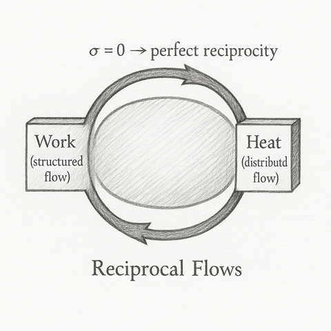
This flow describes the dual nature of work and heat as reciprocal boundary exchanges within a coherent energy field. Where classical thermodynamics treats them as separate modes of energy transfer, Flow Algebra unifies them as paired channels of coherence: one structured (work), one distributed (heat). They are not different in substance, but in symmetry — work is directional ordering of field tension, while heat is the same energy diffused through phase-space microstates.
Conceptual Core
At the heart of the model lies the First and Second Laws of thermodynamics re-expressed as flow invariants:
Here, andS evolve together — energy and entropy forming a coupled pair. In Holographic terms, this expresses the boundary’s coherence gradient: when alignment is perfect (σ → 0), energy exchange is reversible and coherent; when alignment fails, part of that tension disperses as entropy — a measurable loss of structural memory.
Reciprocity and Symmetry
Using Onsager’s framework, the flow defines cross-coupled responses between mechanical and thermal channels:
with the reciprocity condition Lqw=Lwq enforcing mirror symmetry of cause and effect. This symmetry is broken only by dissipation (σ > 0), representing coherence loss through microscopic uncertainty or boundary scattering. Thus, work and heat are reversible mirrors of one another in the coherence limit.
Boundary Coherence Index (IB)
To quantify how reversible an exchange is, the flow introduces IB ∈ [0, 1], the boundary coherence index:
IB = 0: incoherent, energy disperses as thermal noise.
This gives engineers and theorists a continuous measure of how “tight” or “loose” an energy boundary behaves, bridging pure thermodynamics with boundary-based coherence geometry.
Interpretation
Work corresponds to structured curvature alignment (pressure–volume, force–velocity, or field–flux pairs), while heat corresponds to distributed curvature relaxation, the system’s way of restoring symmetry after deformation. Together they form a single feedback loop:
Work converts ordered boundary tension into motion.
Heat returns dispersed curvature to equilibrium.
This cycle is the reciprocal heartbeat of every physical system — from engines and phase transitions to biological metabolism and neural computation.
In the HST View
In Holographic Space-Time, this reciprocity arises because every boundary exchange seeks to conserve total coherence. The Lorentz curvature of motion and the thermal curvature of memory are not distinct forces, but dual projections of the same field geometry. Work and heat are therefore the vector and scalar components of a unified energy flow, maintaining the equilibrium between form and information.
Applications and Extensions
Modelling reversible engines and finite-time thermodynamic cycles
Studying entropy production in materials, plasmas, or information systems.
Analysing AI processor thermals and feedback coherence at micro-architectural level.
Linking mechanical work, radiation, and computation through a single energy-flow syntax.
Connection to the Finite-Time Engine Flow
The Work and Heat — Reciprocal Flows model defines the local symmetry that governs every reversible exchange. The Finite-Time Engine flow builds upon this foundation by introducing timing, loss, and boundary asymmetry — showing what happens when those reciprocal channels are no longer perfectly aligned.
In that later model, the coherence index (IB) and conductances (Gₕₒₜ, Gₐₗₒₗd) determine how closely each stroke adheres to the reciprocal ideal defined here. When IB → 1 and thermal gradients shrink, the engine approaches the reversible limit described by this flow. When IB falls, dissipation rises, and the symmetry between work and heat fractures — entropy production becomes visible as measurable loss of coherence.
Thus, these two flows form a natural pair:
This flow — the universal law of reciprocity and energy balance.
Finite-Time Engine — the temporal expression of that law under finite coherence and real-world constraints.
Together, they outline the bridge between thermodynamic theory and dynamic coherence geometry — a continuous spectrum from reversible symmetry to dissipative reality.