flow "Universal Gravitation as Boundary Stress" v1.0

# ---------- PURPOSE ----------
# Recast Newtonian gravitation as a boundary-stress flow.
# Gravity is expressed via a scalar potential Φ and field g = -∇Φ, with a
# gravitational stress tensor carrying momentum/pressure on boundaries.
# A coherence index (IB) encodes how ideally the boundary transmits curvature (IB=1 → ideal).
# Supports 2-body dynamics, N-body superposition, Gauss/Poisson relations, and loss heuristics.

# ---------- PARAMETERS ----------
params:
  units: "SI"
  G: 6.67430e-11            # gravitational constant [m^3 kg^-1 s^-2]
  IB: 0.0..1.0 = 1.0        # boundary coherence (1 = ideal Newtonian limit)
  softening_eps: 1.0e-3     # [m] softening radius to avoid singular forces in demos
  include_stress: true      # expose gravitational stress tensor and energy density
  loss_coeff: 0.0           # optional coherence-loss (phenomenological) [s^-1]
  dt: 0.0?                  # optional integrator step hint (for scenes)

# ---------- STATE ----------
# Minimal 2-body plus field form; engines can extend to N bodies with arrays.
state Body1:
  m: positive               # mass [kg]
  r: vec3                   # position [m]
  v: vec3                   # velocity [m/s]
  a: vec3                   # acceleration [m/s^2]

state Body2:
  m: positive
  r: vec3
  v: vec3
  a: vec3

state Field:
  r12: vec3                 # r2 - r1
  R:   positive             # |r12|
  u:   vec3                 # unit vector r12 / R
  Phi1: real                # potential at body 1 due to 2
  Phi2: real                # potential at body 2 due to 1
  g1:   vec3                # field at 1 due to 2
  g2:   vec3                # field at 2 due to 1

state Integrals:
  L: vec3                   # total angular momentum [kg m^2/s]
  E: real                   # total mechanical energy [J]
  E_dot_loss: real          # phenomenological loss rate [W]

# Optional continuum form (for Gauss/Poisson and stress)
state Continuum?:
  rho: real                 # mass density [kg/m^3]
  Phi: real                 # potential [m^2/s^2]
  g:   vec3                 # field = -∇Φ [m/s^2]
  u_g: real                 # energy density [J/m^3]
  T_g[3][3]: real           # gravitational stress tensor [Pa]

# ---------- INVARIANTS (FIELD + FORCES) ----------
invariants:

  # Geometry
  Field.r12 = Body2.r - Body1.r
  Field.R   = max(norm(Field.r12), params.softening_eps)
  Field.u   = Field.r12 / Field.R

  # Point-mass potentials and fields (IB scales boundary coherence)
  Field.Phi1 = - params.IB * params.G * Body2.m / Field.R
  Field.Phi2 = - params.IB * params.G * Body1.m / Field.R

  Field.g1 = -∇Φ_at_1 ≡  params.IB * params.G * Body2.m / (Field.R^2) * Field.u     # accel on 1 toward 2
  Field.g2 =  -Field.g1 * (Body1.m / Body2.m)                                        # equal & opposite per unit mass

  # Newton's 2nd law with softened inverse-square
  Body1.a =  Field.g1
  Body2.a = -params.IB * params.G * Body1.m / (Field.R^2) * Field.u

  # Mechanical energy (two-body)
  Integrals.E = 0.5*Body1.m*dot(Body1.v,Body1.v) + 0.5*Body2.m*dot(Body2.v,Body2.v)
                + Body1.m*Field.Phi1             + Body2.m*Field.Phi2

  # Angular momentum (about origin)
  Integrals.L = Body1.m * cross(Body1.r, Body1.v) + Body2.m * cross(Body2.r, Body2.v)

  # Phenomenological coherence-loss channel (optional)
  Integrals.E_dot_loss = - params.loss_coeff * (abs(Integrals.E))
  # Engines may apply: dE/dt += E_dot_loss, dv/dt adjusted along v̂ to mimic tiny drag-like loss

  # Continuum relations (for field pages / Gauss / Poisson)
  if defined(Continuum):
    # Gauss law for gravity: ∮ g·dA = -4π G M_enclosed  (sign opposite to electrostatics)
    # Poisson equation:
    laplacian(Continuum.Phi) = 4*pi*params.G*Continuum.rho
    Continuum.g = -grad(Continuum.Phi)

    if params.include_stress:
      # Gravitational energy density and stress (Newtonian field-theory heuristic)
      Continuum.u_g = - (norm(Continuum.g)^2) / (8*pi*params.G)
      # Tij = -(1/4πG)(g_i g_j - 1/2 |g|^2 δ_ij)
      for i in [0,1,2]:
        for j in [0,1,2]:
          Continuum.T_g[i][j] = - (1/(4*pi*params.G)) * (Continuum.g[i]*Continuum.g[j] - 0.5*norm(Continuum.g)^2 * (i==j))

# ---------- TRANSFORMS ----------
transforms:

  # Leapfrog/Euler step (engine can pick integrator; provided for demo scenes)
  step_dynamics (when params.dt > 0):
    Body1.v += Body1.a * params.dt
    Body2.v += Body2.a * params.dt
    Body1.r += Body1.v * params.dt
    Body2.r += Body2.v * params.dt
    # apply tiny coherence-loss power if enabled (align along velocity directions)
    if params.loss_coeff > 0 and Integrals.E > 0:
      Body1.v *= (1 - 0.5*params.loss_coeff*params.dt)
      Body2.v *= (1 - 0.5*params.loss_coeff*params.dt)

  # Two-body reduction (diagnostic): μ, M, specific energy ε, specific ang. mom h
  kepler_reduction:
    M  = Body1.m + Body2.m
    mu = params.G * M * params.IB
    r  = Field.R
    v_rel = norm(Body2.v - Body1.v)
    eps_spec = 0.5*v_rel^2 - mu / r            # < 0 bound, =0 parabolic, >0 hyperbolic
    h_vec = cross(Field.r12, (Body2.v - Body1.v))
    h = norm(h_vec)

  # Escape speed at radius r (ideal IB=1)
  escape_speed:
    v_esc = sqrt( 2 * params.IB * params.G * (Body1.m + Body2.m) / Field.R )

# ---------- MONITORS ----------
monitors:
  symmetry_newton_third:
    # For ideal IB, forces equal/opposite
    F1 = Body1.m * Body1.a
    F2 = Body2.m * Body2.a
    if params.IB == 1:
      assert norm(F1 + F2) <= 1e-9

  invariants_ideal:
    if params.IB == 1 and params.loss_coeff == 0:
      dL = d/dt(Integrals.L)
      dE = d/dt(Integrals.E)
      assert norm(dL) <= 1e-9
      assert abs(dE) <= 1e-9

  field_equations:
    if defined(Continuum):
      # sanity: g ≈ -∇Φ
      assert norm(Continuum.g + grad(Continuum.Phi)) <= 1e-6

# ---------- SCENES ----------
scenes:

  circular_orbit_demo:
    given params:
      IB: 1.0
      dt: 0.01
    given Body1:
      m: 5.97e24
      r: [0,0,0]
      v: [0,0,0]
    given Body2:
      m: 1000
      r: [7.0e6, 0, 0]
      v: [0, 7546.0, 0]     # ~circular around Earth at ~7e6 m
    enable:
      - step_dynamics
      - kepler_reduction
    expect:
      near_constant_R: abs(Field.R - 7.0e6) << 1e4
      energy_bound: Integrals.E < 0
      comment: "Stable circular orbit; L and E conserved (IB=1)."

  radial_free_fall:
    given params:
      IB: 1.0
      dt: 0.02
    given Body1:
      m: 5.97e24
      r: [0,0,0]
      v: [0,0,0]
    given Body2:
      m: 10
      r: [1.0e7, 0, 0]
      v: [0, -100, 0]
    enable: [step_dynamics]
    expect:
      R_decreases: d/dt(Field.R) < 0
      v_growth:    norm(Body2.v) increases

  escape_velocity_check:
    given:
      r0 = 6.4e6
      M  = 5.97e24
    compute:
      v_esc = sqrt(2 * params.IB * params.G * M / r0)
    expect:
      v_esc ≈ 11186  # m/s for IB=1, Earth radius

  weak_field_sheet (continuum):
    given Continuum:
      rho: 5510      # kg/m^3 (proxy region)
      Phi: undefined
    note: "Engines may solve ∇^2Φ = 4πGρ on a grid; u_g and T_g then become available."

# ---------- NOTES ----------
notes:
  - Point-mass law (coherent boundary): \( \mathbf{F}_{12} = -\,\hat{\mathbf{r}}\,\dfrac{G\,m_1 m_2}{r^2} \);
    here scaled by \(I_B\) to encode ideal vs. imperfect curvature transmission.
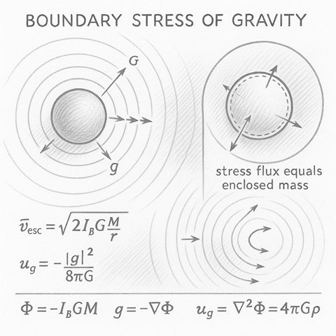
  - Potential & field: \( \Phi = -\,I_B\,G M / r,\quad \mathbf{g} = -\nabla \Phi \).
  - Gauss/Poisson: \( \oint \mathbf{g}\cdot d\mathbf{A} = -4\pi G M_{\text{enc}},\quad \nabla^2 \Phi = 4\pi G \rho \).
  - Stress view (Newtonian field heuristic): energy density \( u_g = -|\mathbf{g}|^2/(8\pi G) \);
    stress \( T_{ij} = -(1/4\pi G)\,(g_i g_j - \tfrac{1}{2}|\mathbf{g}|^2 \delta_{ij}) \);
    surface integrals of \(T_g\) transmit gravitational momentum as *boundary stress*.
  - Two-body reductions: specific energy \( \epsilon = v^2/2 - \mu/r \) with \( \mu = I_B G(m_1+m_2) \).
  - Coherence loss (optional): a tiny \( \dot E = -\lambda |E| \) can emulate out-of-model leaks;
    set loss_coeff=0 for pure Newtonian invariants.
  - Softening \( \epsilon \) is a numerical guard; reduce for high-accuracy analytics.
Overview
Gravity can be read as boundary stress: curvature tension stored in a scalar potential whose gradient transmits momentum through space. In this view, masses shape a coherent field; boundaries (surfaces around masses) feel stress from that field, and motion follows the resulting pressure of curvature.
A coherence index measures how ideally the boundary transmits that curvature: is the Newtonian ideal; encodes tiny departures (loss, scattering, unresolved structure).
Surface integrals of over a closed boundary transmit momentum — gravity as pressure of curvature. Gauss/Poisson close the picture:
$$ \oint \mathbf{g} \cdot d\mathbf{A} = -4\pi G M_{\mathrm{enc}}, \qquad \nabla^2 \Phi = 4\pi G \rho. $$
🔁 Conserved Structure (Ideal vs. Coherence-limited)
For and no losses, the two-body system conserves:
$$ d\mathbf{L} = 0, \qquad \frac{dE}{dt} = 0. $$
With small coherence loss (phenomenological ), orbits slowly spiral and energy drains along — a controlled deviation useful for demos but set for the pure Newtonian limit.
🧩 HST Interpretation
Mass imprints a curvature map on the boundary of space;
Gravity is the stress required to maintain that map across distances;
Motion is the natural slide along the gradient of that stress. measures how perfectly the boundary remembers this map: perfect memory gives the exact inverse-square law; imperfect memory manifests as tiny departures or effective drag in reduced models.
🔬 What to Explore (Scenes)
Circular orbit demo: shows and conservation when .
Free-fall: potential kinetic conversion along .
Escape check: verify at a chosen radius.
Continuum sheet: solve to visualise and .
🧠 Summary
Gravity, in this language, is coherent curvature pressure carried by a scalar potential. Boundaries transmit that pressure as stress; motion follows the gradients; Gauss and Poisson guarantee global consistency. With we recover Newton cleanly; with we gain a dial for tiny, controlled departures — a practical bridge between ideal geometry and real boundaries.