Chapter 15
Continuous ↔ Discrete Equivalence
Meta-Principles of Coherence Physics
Author: Mark Anthony Higgins
Revised Date: 23 February 2026
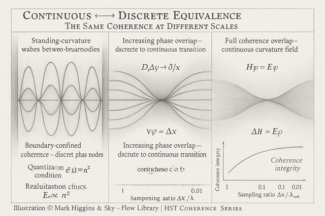
Continuous_Discrete_Equivalence redefines the long-standing divide between continuous and discrete physics.
Rather than two competing descriptions, they are two sampling resolutions of the same coherence field.
In HST, discreteness appears whenever a boundary constrains coherence into closed loops, forming quantised phase nodes.
Continuity arises when those loops overlap and the curvature field becomes smooth.
Both obey the same operator equations and conservation laws — only the coherence ratio
\[ \frac{\lambda_{\mathrm{coh}}}{\Delta x} \]
decides whether the system appears quantised or continuous.
Every physical system is built from coherence loops — self-consistent oscillations of curvature and phase.
When the sampling scale (Δx) used to describe a system becomes comparable to the coherence wavelength
\[ \lambda_{\mathrm{coh}} \]
each loop resolves as an independent state: the system becomes discrete.
When Δx is much smaller than λ₍coh₎, adjacent loops overlap; the boundary between them disappears — the system appears continuous.
In this view, discreteness and continuity are not fundamental categories but perspectives of resolution:
geometry quantised by boundary conditions, or geometry blurred by phase overlap.
Start from the finite-difference form of a derivative:
\[ D_{\Delta x}\psi = \frac{\psi(x + \Delta x) - \psi(x - \Delta x)}{2\,\Delta x}\,. \]
As Δx → 0, this converges smoothly to the continuous derivative:
\[ D\psi = \frac{\partial \psi}{\partial x}\,. \]
The governing equation,
\[ H\psi = E\psi\,. \]
is the same in both forms.
What changes is the domain and boundary condition:
Quantisation arises whenever coherence loops close on themselves:
\[ \oint p\,dx = n h\,. \]
Continuity emerges when coherence is unbounded or densely sampled.
\[ \oint p\,dx = n\,h\,. \]
Continuity emerges when coherence is unbounded or densely sampled.
| Aspect | Discrete regime | Continuous regime | Unified view |
|---|---|---|---|
|
Boundary
|
Finite / closed
|
Open / overlapping
|
Same curvature field
|
|
Coherence ratio
|
Δx/λ₍coh₎ ≳ 1
|
Δx/λ₍coh₎ ≪ 1
|
Governs apparent regime
|
|
Spectrum
|
Quantised {Eₙ}
|
Continuous
|
Same operator, different domain
|
|
Wavefunctions
|
Localised modes ψₙ
|
Smooth ψ(x)
|
Fourier-related bases
|
|
Coherence integrity
|
Lower (<1)
|
Higher (≈1)
|
Degree of phase overlap
|
The transition between regimes is perfectly smooth.
As phase overlap increases, the discrete nodes blur into continuous curvature —
exactly the same mathematics seen through different coherence sampling.
In HST, quantisation is a boundary phenomenon.
When coherence is trapped between reflective boundaries (atomic orbitals, resonant cavities, standing curvature waves),
the allowed modes are constrained to fit integer multiples of λ₍coh₎ —
geometry literally counting its own phase wraps.
When the boundary opens or overlaps globally, coherence is no longer confined to integer resonance.
The field becomes continuous; energy varies smoothly, and quantised transitions merge into flow.
Thus, the discrete-to-continuous transition is not a breaking of law but the re-opening of boundary coherence.
The total curvature energy,
\[ E_{\mathrm{total}} \propto \int |\psi|^{2}\, dV\,. \]
is conserved in both cases; only its representation changes.
In the discrete view, the integral collapses to a sum over nodes:
\[ E_{\mathrm{total}} = \sum_{n} E_{n}\,|\psi_{n}|^{2}\,. \]
In the continuum limit, this sum becomes an integral once again.
No physical step occurs between them — only a change of description as the coherence field is sampled more finely.
The universe, then, is not discrete or continuous, but continuously discrete —
a lattice of coherence so fine that it behaves as a smooth geometry, yet with phase structure that can count itself when observed closely.
This flow completes the Meta-Principles of Coherence Physics by showing that discreteness, continuity, and quantisation are sampling perspectives on a single geometric law.
Quantum jumps, classical continua, and wave equations all emerge from one coherence engine —
differing only by how finely the boundary resolves itself.
It dissolves the last illusion of separation between quantum and classical, particle and field, discrete and continuous.
All are one curvature system, seen at different scales of resolution.
Discreteness is coherence counted; continuity is coherence seen too closely to count.
Both are the same geometry, written at different resolutions of truth.