
Chapter 22
Lorentz Force and Boundary Interaction

Field and Energy Systems
Author: Mark Anthony Higgins
© Mark Anthony Higgins 11 October 2025
Revised Date: 23 February 2026
Audio Overview
Flow Algebra
flow "LorentzForce_BoundaryInteraction"

# ---------- STATES ----------
state:
  # particle
  particle.q: float                    # charge (C)
  particle.m: float                    # rest mass (kg)
  particle.x: vec[float,3]             # position (m)
  particle.v: vec[float,3]             # velocity (m/s)
  particle.p: vec[float,3]             # momentum (kg·m/s)
  particle.gamma: float                # relativistic factor γ
  particle.energy.K: float             # kinetic energy (J)

  # fields at particle
  field.E: vec[float,3]                # electric field E(x,t) (V/m)
  field.B: vec[float,3]                # magnetic field B(x,t) (T)
  field.grad: tensor                   # local gradients (for boundary estimates)

  # forces / power
  force.F: vec[float,3]                # Lorentz force
  power.P: float                       # power delivered to particle = q E·v
  reaction.radiation.P_rad: float      # radiated power (Larmor/relativistic)
  reaction.radiation.f_rad: vec[float,3] # effective radiation-reaction force (approx)

  # boundary model
  boundary.type: "none"|"conductor"|"dielectric"
  boundary.surface.S: surface          # implicit/parametric surface
  boundary.normal.n: fn(vec3)->vec3    # outward unit normal
  boundary.εr: float                   # relative permittivity (dielectric)
  boundary.μr: float                   # relative permeability (dielectric)
  boundary.image.enabled: bool         # use image-method when applicable
  boundary.integrity: float            # 0..1 coherence of boundary-field coupling

  # energy–momentum accounting
  poynting.S: vec[float,3]             # local Poynting vector (W/m^2)
  stress.T: tensor                     # Maxwell stress tensor at boundary patch
  work.exchange.W: float               # accumulated work by fields (J)
  time.t: float

# ---------- PARAMETERS ----------
params:
  c: 2.998e8
  ε0: 8.8541878128e-12
  μ0: 4π×10^-7
  dt: float
  use_relativistic: bool
  radiation.reaction: "none"|"Larmor_NR"|"LandauLifshitz"
  boundary.image_plane.z0: float       # plane z = z0 (for simple image model)
  friction.eta: float                  # optional phenomenological drag

# ---------- INVARIANTS ----------
invariant:
  - force.F = particle.q * ( field.E + cross(particle.v, field.B) )
  - power.P = particle.q * dot(field.E, particle.v)        # B-part does no work
  - relativistic:
      particle.gamma = 1 / sqrt(1 - |v|^2 / c^2)
      particle.p = particle.gamma * particle.m * particle.v
      particle.energy.K = (particle.gamma - 1) * particle.m * c^2
  - nonrelativistic:
      particle.p = particle.m * particle.v (if !use_relativistic)
      particle.energy.K = 0.5 * particle.m * |v|^2
  - radiation (nonrelativistic Larmor): P_rad = (q^2 a^2) / (6π ε0 c^3)
  - momentum balance (schematic): d(particle.p)/dt = force.F + reaction.radiation.f_rad - η v
  - boundary jump conditions:
      conductor:  E_tan = 0 on S,  B_norm = 0 on S
      dielectric: ε1 E_norm(1) = ε2 E_norm(2),  B_tan continuous (μ1, μ2)
  - coherence continuity: ∂μ J_coh^μ = 0 ↔ work by fields + stress flux = particle energy–momentum change

# ---------- TRANSFORMS ----------
transform:

  sample_fields_at_particle:
    do:
      field.E = E_at(particle.x, time.t)
      field.B = B_at(particle.x, time.t)
      field.grad = field_gradients_near(particle.x, time.t)

  compute_lorentz_force:
    do:
      force.F = particle.q * ( field.E + cross(particle.v, field.B) )
      power.P = particle.q * dot(field.E, particle.v)

  radiation_reaction_update:
    do:
      if params.radiation.reaction == "Larmor_NR":
        a = (force.F / particle.m)         # NR estimate
        reaction.radiation.P_rad = (particle.q**2 * |a|**2) / (6π*params.ε0*params.c**3)
        reaction.radiation.f_rad = - reaction.radiation.P_rad * particle.v / max(|particle.v|^2, 1e-12)
      elif params.radiation.reaction == "LandauLifshitz":
        # compact LL approximation (symbolic placeholder)
        reaction.radiation.f_rad = landau_lifshitz_force(particle, field.E, field.B, params)
        reaction.radiation.P_rad = dot(reaction.radiation.f_rad, particle.v)
      else:
        reaction.radiation.P_rad = 0
        reaction.radiation.f_rad = [0,0,0]

  update_momentum_velocity:
    do:
      F_total = force.F + reaction.radiation.f_rad - params.friction.eta * particle.v
      if params.use_relativistic:
        # dp/dt = F_total ; p = γ m v → update v via iterative step
        particle.p += F_total * params.dt
        particle.gamma = 1 / sqrt(1 - |particle.v|^2 / params.c^2)
        particle.v = relativistic_v_from_p(particle.p, particle.m, params.c)
      else:
        particle.v += (F_total / particle.m) * params.dt
        particle.p = particle.m * particle.v
      particle.x += particle.v * params.dt
      particle.energy.K = (particle.gamma - 1)*particle.m*params.c**2 if params.use_relativistic else 0.5*particle.m*|particle.v|**2
      work.exchange.W += power.P * params.dt

  boundary_interaction:
    pre:
      require boundary.type != "none"
    do:
      # detect approach/crossing & enforce jump conditions/coherence
      if intersects(boundary.surface.S, particle.x):
        if boundary.type == "conductor":
          # enforce E_tan ≈ 0 at S via image or reflection of tangential component
          field.E = project_normal(field.E, boundary.normal.n(particle.x))
          # simple image-method for infinite plane z = z0
          if boundary.image.enabled and is_plane_z(boundary.surface.S, params.boundary.image_plane.z0):
            particle_image = { q: -particle.q, x: mirror_z(particle.x, params.boundary.image_plane.z0) }
            field.E += E_of_point_charge(particle_image.q, particle_image.x, particle.x)
        elif boundary.type == "dielectric":
          (E1n,E1t) = split_normal_tan(field.E, boundary.normal.n(particle.x))
          ε1 = params.ε0 * 1.0; ε2 = params.ε0 * boundary.εr
          E2n = (ε1/ε2) * E1n
          field.E = combine_normal_tan(E2n, E1t)
      # compute stress & impulse on boundary patch for bookkeeping
      stress.T = maxwell_stress(field.E, field.B, params.ε0, params.μ0)
      # optional: adjust boundary.integrity by stress surge
      boundary.integrity = clamp(boundary.integrity - stress_intensity(stress.T), 0, 1)

  update_poynting_stress:
    do:
      poynting.S = (1/params.μ0) * cross(field.E, field.B)
      # optional logging of momentum exchange with boundary via stress tensor flux

  tick:
    do:
      time.t += params.dt

# ---------- MONITORS ----------
monitor:
  lorentz_power:
    observe: [power.P]
    report: "Power to particle qE·v; magnetic part does no work."

  kinematics:
    observe: [particle.x, particle.v, particle.energy.K, particle.gamma]
    report: "Tracks trajectory and kinetic energy (relativistic if enabled)."

  radiation_balance:
    observe: [reaction.radiation.P_rad]
    report: "Radiative loss estimate (Larmor/LL) for accelerated charges."

  boundary_conditions:
    observe: [boundary.type, boundary.integrity]
    report: "Enforces E_tan=0 on conductors, normal/tangential continuity on dielectrics; logs stress on S."

  coherence_continuity:
    observe: [poynting.S]
    report: "Energy–momentum exchange: Poynting flux + stress ↔ particle/boundary updates (∂μJ_coh^μ=0)."

# ---------- NOTES (coherence view) ----------
note:
  - The Lorentz force is the **local curvature push** on a charge: phase gradient (E) plus twist coupling (v×B).
  - Work transfer is purely via E:  P = q E·v ;  B redirects motion without doing work — **coherence rotates, not adds energy**.
  - Radiation reaction accounts for **coherence shedding** when acceleration is nonzero; Larmor/LL give practical estimates.
  - Boundaries encode coherence constraints:
      • **Conductor:** E_tangential→0, induced surface currents/charges restore coherence; image methods approximate global correction.
      • **Dielectric:** normal D and tangential E/B continuity maintain **phase consistency** across media.
  - Maxwell stress & Poynting flux capture momentum/energy passed to boundaries; no energy is lost, only **redistributed** (∂μJ_coh^μ = 0).
  - Relativistic option keeps dynamics consistent at high |v|/c via γ, p = γmv, ensuring **coherence-causal** motion.
What this flow captures

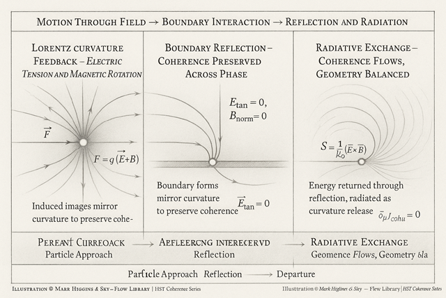
LorentzForce_BoundaryInteraction describes how a charged particle interacts with the electromagnetic field and with physical boundaries — conductors, dielectrics, or coherent surfaces — through curvature-phase feedback.
In classical form, the Lorentz force

\[ \mathbf{F} = q\,(\mathbf{E} + \mathbf{v} \times \mathbf{B})\,. \]

gives the instantaneous push on a charge due to electric and magnetic fields.
In HST, this same relation describes how local curvature gradients (E) and curvature twists (B) redirect a charge’s motion while preserving overall coherence.

The boundary of space around the particle acts as a curvature interface: energy, momentum, and phase flow continuously through it without loss, obeying

<\[ \partial_{\mu} J^{\mu}_{\mathrm{coh}} = 0\,. \]

This is not simply “force through a field,” but geometry reorganising itself to maintain continuity as curvature interacts with curvature.


Core intuition (HST view)

Electric and magnetic fields are local expressions of curvature tension and rotation.
When a charge moves, it deforms this curvature; when curvature changes, it guides the charge’s motion.
The interaction is fully reciprocal — a coherence exchange, not a one-way influence.

  • Electric field (E): the local phase gradient — curvature tension pushing the particle directly.
  • Magnetic field (B): curvature twist — it redirects motion orthogonally, changing direction but not speed.
  • Lorentz force: geometry steering geometry, ensuring curvature flow and phase motion remain synchronised.

Boundaries reinforce this same continuity: the electromagnetic field adjusts its configuration (surface charge, current, or polarisation) so that phase coherence remains unbroken across the interface.


Mathematical structure

Lorentz force and energy balance

\[ \mathbf{F} = q\,(\mathbf{E} + \mathbf{v} \times \mathbf{B}), \qquad P = q\,\mathbf{E} \!\cdot\! \mathbf{v}\,. \]

Magnetic forces redirect momentum but perform no work; energy transfer arises only from the electric component.

Kinetic energy follows

\[ \frac{dK}{dt} = q\,\mathbf{E} \!\cdot\! \mathbf{v}\,. \]

Relativistically,

\[ \mathbf{p} = \gamma\,m\,\mathbf{v}, \qquad K = (\gamma - 1)\,m\,c^{2}\,. \]

Radiation reaction

Accelerating charges radiate coherence as electromagnetic waves.
The Larmor expression gives the non-relativistic loss:

\[ P_{\mathrm{rad}} = \frac{q^{2} a^{2}}{6\pi\,\varepsilon_{0}\,c^{3}}\,. \]

This represents coherence leakage — stored curvature tension converting into propagating geometry.
In equilibrium, radiation reaction ensures global continuity: energy is conserved, but redistributed.

Boundary interaction

At a conducting surface:

\[ E_{\mathrm{tan}} = 0, \qquad B_{\mathrm{norm}} = 0\,. \]

At a dielectric interface:

\[ \varepsilon_{1} E_{\mathrm{norm,1}} = \varepsilon_{2} E_{\mathrm{norm,2}}, \qquad B_{\mathrm{tan,1}} = B_{\mathrm{tan,2}}\,. \]

These are not arbitrary constraints but coherence rules: the boundary enforces phase matching between internal and external curvature fields.

When a charge approaches a conductor, an image charge forms — the field’s way of mirroring phase curvature to maintain boundary symmetry.
The result is not attraction or repulsion by “method,” but a geometric reflex ensuring field continuity.


Energy and momentum continuity

The Poynting vector and Maxwell stress tensor link field flow and mechanical reaction:

\[ \mathbf{S} = \frac{1}{\mu_{0}}\,(\mathbf{E} \times \mathbf{B}), \qquad \frac{\partial u}{\partial t} + \nabla \!\cdot\! \mathbf{S} = -\,\mathbf{J}\!\cdot\!\mathbf{E}\,. \]

\[ \mathbf{T} = \varepsilon_{0}\!\left( \mathbf{E}\mathbf{E} - \tfrac{1}{2}E^{2}\mathbf{I} \right) + \frac{1}{\mu_{0}}\!\left( \mathbf{B}\mathbf{B} - \tfrac{1}{2}B^{2}\mathbf{I} \right). \]

Momentum carried by the fields passes into matter through T\mathbf{T}; energy through S\mathbf{S}.

\[ \partial_{\mu} J^{\mu}_{\mathrm{coh}} = 0\,. \]

signifying that curvature energy is neither created nor destroyed — only redirected between particle, field, and boundary.


Interpretation in coherence physics

Classical conceptHST reinterpretation
Lorentz force
Curvature phase pressure and twist feedback
Work by E-field
Conversion of curvature tension into particle motion
Magnetic deflection
Rotational coherence conserving kinetic energy
Radiation reaction
Curvature feedback releasing coherence as light
Conducting boundary
Phase mirror enforcing coherence continuity
Dielectric boundary
Partial coherence coupling between two curvatures
Poynting flux
Flow of coherence energy through space

Thus, electromagnetic interaction is the contact surface of coherence itself — the interface between motion and memory.


Boundary coherence and integrity

The boundary’s integrity parameter (IBI_{B}) measures how perfectly it maintains coherence continuity:

  • \( I_{B} = 1:\; \text{perfect reflection or transmission — no coherence loss.} \)
  • \( I_{B} < 1:\; \text{partial loss — radiation or absorption.} \)
  • \( I_{B} = 0:\; \text{incoherent surface — phase destroyed, converted to heat or noise.} \)

Good conductors restore coherence by reflecting phase (image charge).
Dielectrics absorb part of the curvature and pass the rest on — translation rather than reflection.
In all cases, coherence strives to minimise phase discontinuity.


Philosophical coherence

The Lorentz force is the micro-expression of geometric fairness:
every curvature disturbance meets an equal response that preserves balance.
Boundaries are not obstacles but mediators of continuity, transforming one field configuration into another without breaking the loop of coherence.

Radiation, reflection, and reaction are therefore the same act seen from different frames:

Geometry remembering where it came from, and adjusting itself to stay whole.


Significance

This flow links the motion of individual charges to the universal coherence system described by Maxwell’s recursion.
It shows that every acceleration, reflection, and field reaction is governed by the same conservation law:

\[ \partial_{\mu} J^{\mu}_{\mathrm{coh}} = 0\,. \]

The Lorentz force is the mechanical language of that law; Maxwell’s equations are its field language; and boundary conditions are its geometric syntax.
Together, they ensure the electromagnetic universe operates as a single recursive coherence network — stable, responsive, and beautifully self-aware.


In essence

The Lorentz force is the push of geometry correcting its own imbalance.
Boundaries are coherence mirrors; radiation is their language of exchange.
Every motion of charge is the field’s way of remembering itself.

Kireth Research
38 Thorndale Croft, Wetwang, Driffield
East Riding of Yorkshire YO25 9XZ
Designed By