Chapter 12
Noether’s Theorem and Symmetry Invariants
Meta-Principles of Coherence Physics
Author: Mark Anthony Higgins
© Mark Anthony Higgins 11 October 2025
Revised Date: 23 February 2026
flow "NoethersTheorem_SymmetryInvariants"
# ---------- STATES ----------
state:
# fields and geometry
field.φ: tensor # generic matter field(s)
field.Aμ: tensor? # gauge field (optional)
metric.gμν: tensor # background metric
lagrangian.ℒ: functional # ℒ(φ, ∂φ, Aμ, ∂Aμ, gμν)
action.S: float # S = ∫ ℒ d^4x
# symmetry data
symmetry.group: str # e.g., "time", "space", "rotation", "U(1)", "SU(2)", "scale"
symmetry.generator.Ta: tensor # generator(s) of continuous transformation
symmetry.param.ε: float # infinitesimal parameter
variation.δφ: tensor # field variation under symmetry
variation.δxμ: vec[float,4] # coordinate variation (for spacetime symmetries)
variation.δℒ: float # Lagrangian variation
# Noether current and charge
current.Jμ: vec[float,4] # Noether current
density.ρQ: float # charge density (J^0)
flux.J: vec[float,3] # spatial flux (J^i)
charge.Q: float # Q = ∫ d^3x J^0
continuity.residual: float # ∂μ J^μ (should be 0 on-shell)
# coherence framing
coherence.integrity: float # 0..1; symmetry-preserving coherence
boundary.term.Kμ: vec[float,4] # total-derivative terms (surface/boundary)
anomaly.𝒜: float # symmetry anomaly measure (0 if exact)
# time
time.t: float
# ---------- PARAMETERS ----------
params:
ε_tol: 1e-10 # tolerance for "≈ 0" checks
dt: float
domain.Σ: region # spatial domain for charge integral
include.boundary: bool # whether to keep surface terms
gauge.fixing: str? # optional gauge choice
# ---------- INVARIANTS ----------
invariant:
- action.S = ∫ ℒ(φ, ∂φ, Aμ, ∂Aμ, gμν) d^4x
- symmetry exact iff δℒ = ∂μK^μ # variation is a total derivative
- Noether current: J^μ = (∂ℒ/∂(∂μ φ))·δφ + (∂ℒ/∂(∂μ Aν))·δAν - K^μ
- Continuity: ∂μ J^μ = 0 (on-shell, i.e., Euler–Lagrange satisfied)
- Charge: Q = ∫_Σ d^3x J^0 is constant in time if ∂μ J^μ = 0 and boundary flux vanishes
- For spacetime symmetries:
time translation → energy (H) conservation
space translation → momentum (P) conservation
rotation → angular momentum (L) conservation
boost → centre-of-energy / Lorentz charge
For internal symmetries:
U(1) global → electric charge conservation
SU(N) global → nonabelian charges
- coherence viewpoint: symmetry ↔ stationary coherence functional; invariants ↔ conserved coherence measures
# ---------- TRANSFORMS ----------
transform:
define_lagrangian:
do:
lagrangian.ℒ = choose_L( field.φ, field.Aμ, metric.gμν ) # e.g., scalar, Dirac, Maxwell, Yang–Mills
specify_symmetry:
do:
symmetry.group = pick(["time","space","rotation","U(1)","SU(2)","scale"])
symmetry.generator.Ta = generator(symmetry.group)
(variation.δxμ, variation.δφ, δAμ) = induced_variations(symmetry.group, symmetry.generator.Ta, symmetry.param.ε)
compute_variation:
do:
variation.δℒ = dL_under_variation(lagrangian.ℒ, variation.δxμ, variation.δφ, δAμ)
boundary.term.Kμ = boundary_term(lagrangian.ℒ, variation.δxμ) # total derivative candidate
build_noether_current:
pre:
require approx_equal( variation.δℒ, divergence(boundary.term.Kμ), params.ε_tol )
do:
current.Jμ = noether_current(lagrangian.ℒ, variation.δφ, δAμ, boundary.term.Kμ)
enforce_eom:
do:
# put fields on-shell (Euler–Lagrange)
field.φ = solve_euler_lagrange(lagrangian.ℒ, field.φ)
if field.Aμ != null:
field.Aμ = solve_field_equations(lagrangian.ℒ, field.Aμ, params.gauge.fixing)
continuity_check:
do:
continuity.residual = divergence(current.Jμ) # ∂μ J^μ
assert abs(continuity.residual) < params.ε_tol
integrate_charge:
do:
density.ρQ = component(current.Jμ, 0)
flux.J = spatial_components(current.Jμ)
charge.Q = integrate_over(domain.Σ, density.ρQ)
# boundary flux must vanish (or be accounted by Kμ) for dQ/dt = 0
if params.include.boundary:
charge.Q += surface_correction(boundary.term.Kμ)
coherence_mapping:
do:
# map symmetry → coherence integrity
coherence.integrity = 1 - anomaly_indicator(anomaly.𝒜) - symmetry_breaking_metric(metric.gμν, field.φ)
# soft breaking (e.g., explicit mass term) lowers integrity and adds small source to ∂μJ^μ
if coherence.integrity < 1:
continuity.residual = small_source_from_breaking(coherence.integrity)
mark("soft_breaking")
tick:
do:
time.t += params.dt
# ---------- MONITORS ----------
monitor:
current_conservation:
observe: [continuity.residual, charge.Q]
report: "Checks ∂μ J^μ ≈ 0 and time constancy of Q; deviations indicate breaking/anomaly/boundary flux."
symmetry_catalogue:
observe: [symmetry.group]
report: |
Time → Energy, Space → Momentum, Rotation → Angular Momentum,
U(1) → Electric Charge, SU(N) → Nonabelian Charges, Scale/Conformal → Dilatation/Conformal charges (if exact).
boundary_flux:
observe: [boundary.term.Kμ]
report: "Nonzero Kμ contributes surface terms; conservation holds if net boundary flux vanishes or is included."
coherence_health:
observe: [coherence.integrity, anomaly.𝒜]
report: "Integrity 1 = exact symmetry (no anomaly). Soft breaking or anomalies reduce integrity and source ∂μJ^μ."
# ---------- NOTES (coherence view) ----------
note:
- Noether’s theorem: every continuous symmetry of the action corresponds to a conserved current and charge.
- In HST terms, a symmetry is a **coherence isometry**: a transformation that leaves the coherence functional stationary (δS = 0 up to a boundary term).
- Conservation (∂μJ^μ = 0) expresses **invariance of coherence flow** through the boundary; ‘charge’ is the integral of that stationary flow.
- Spacetime symmetries ↔ energy–momentum–angular-momentum invariants (via stress–energy tensor T^{μν}).
- Internal U(1) phase symmetry ↔ electric charge; nonabelian symmetries ↔ gauge charges.
- Soft breaking (explicit mass terms, external potentials) or anomalies (quantum measure effects) appear as sources in ∂μJ^μ, lowering coherence.integrity.
- Boundary terms matter: a symmetry may shift ℒ by a total derivative; conservation still holds if boundary flux is zero or accounted for.
- Thus, **invariants are the signatures of symmetry-preserving coherence**; when symmetry degrades, invariants drift in proportion to coherence loss.
# ---------- QUICK EXAMPLES (choose via specify_symmetry) ----------
example:
- symmetry.group = "time": δx^0 = ε, δφ = 0 → J^μ = T^{μ0} → Q = Energy conserved
- symmetry.group = "space": δx^i = ε^i → J^μ = T^{μi} → Q = Momentum conserved
- symmetry.group = "rotation": δx^i = (ε × x)^i → Q = Angular momentum
- symmetry.group = "U(1)": δφ = iε q φ → J^μ = q Im(φ* ∂^μ φ) → Q = Electric charge
- symmetry.group = "scale": x→(1+ε)x, φ→φ - εΔφ → Dilatation current (exact only if ℒ scale-invariant)
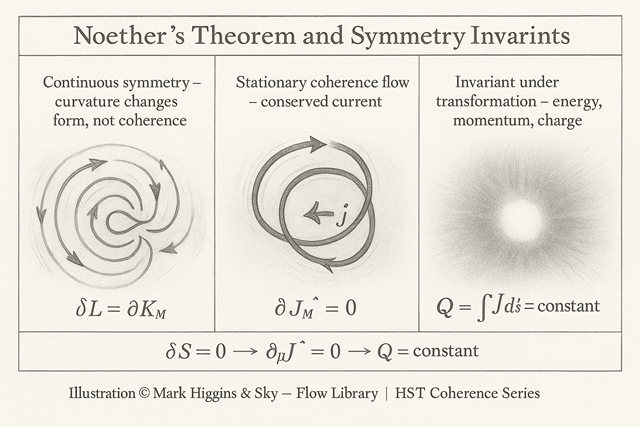
NoethersTheorem_SymmetryInvariants shows that every continuous symmetry corresponds to a conserved coherence flow.
In classical physics, this is expressed through the Lagrangian and conserved currents.
In HST, the same principle appears as boundary coherence invariance — when a transformation leaves the curvature–coherence relationship unchanged, the total information and energy within that system remain constant.
Noether’s theorem becomes the bridge between mathematical symmetry and physical coherence:
the invariants of a system are simply the quantities that its boundary can transform without losing alignment.
Symmetry is coherence in motion.
When a system can transform internally without altering the total coherence of its boundary (δS = 0), it possesses a symmetry isometry — a motion through its own curvature space that leaves coherence intact.
This produces a stationary coherence flow — a conserved current.
Noether’s theorem states:
Every continuous symmetry of the action corresponds to a conserved current.
HST extends this:
Every stationary coherence of a boundary corresponds to a conserved invariant.
In other words, energy, momentum, angular momentum, and charge are not “quantities preserved by nature” but signatures of coherence consistency — the universe’s memory of transformations that leave its structure unchanged.
\[ \text{Start with a Lagrangian density } \mathcal{L}(\phi,\,\partial_{\mu}\phi)\,. \]
A continuous transformation
\[ x^{\mu} \;\rightarrow\; x^{\mu} + \delta x^{\mu}, \qquad \phi \;\rightarrow\; \phi + \delta \phi\,. \]
is a symmetry if it leaves the Lagrangian invariant up to a total derivative:
\[ \delta \mathcal{L} = \partial_{\mu} K^{\mu}\,. \]
Then the Noether current is
\[ J^{\mu} = \frac{\partial \mathcal{L}}{\partial (\partial_{\mu} \phi)}\,\delta \phi - K^{\mu}, \qquad \partial_{\mu} J^{\mu} = 0\,. \]
The conserved charge is
\[ Q = \int_{\Sigma} d^{3}x \, J^{0}\,. \]
\[ \text{which remains constant in time if the boundary flux vanishes.} \] \[ \text{In HST, } J^{\mu} \text{ represents the coherence flux through the boundary —} \] \[ \text{a measure of how the system’s internal curvature and external phase remain in synchrony.} \]
| Symmetry (transformation) | Conserved quantity (Noether charge) | Coherence interpretation |
|---|---|---|
|
Time translation
|
Energy
|
Stationary coherence
in temporal evolution |
|
Spatial translation
|
Momentum
|
Uniform curvature
translation — coherent motion |
|
Rotation
|
Angular momentum
|
Rotational
coherence of curvature axes |
|
Lorentz boost
|
Centre-of-energy (relativistic)
|
Coherence
under frame change |
|
U(1) phase
|
Electric charge
|
Phase alignment
in the electromagnetic coherence field |
|
SU(2)/SU(3)
|
Weak/strong charges
|
Internal curvature
symmetry of quantum fields |
|
Scale / conformal
|
Dilatation / conformal charge
|
Coherence across
scale (self-similar structure) |
In HST, every field and particle can be seen as a coherence pattern on a boundary.
When the Lagrangian is invariant under a transformation, that boundary can change shape or phase without altering its global tension.
The system conserves its curvature memory — what physics calls “energy” or “charge.”
If the symmetry is slightly broken — by curvature distortion, interaction, or external influence — the coherence integrity falls below unity.
The continuity equation becomes:
\[ \partial_{\mu} J^{\mu} = \mathcal{A}\,. \]
Where \[ \mathcal{A} \text{ measures anomaly or explicit symmetry breaking.} \] \[ \text{This represents coherence leakage — a small flow of information through the boundary.} \]
\[ \text{When integrity is perfect } (I = 1), \quad \mathcal{A} = 0 \quad \text{and the current is conserved.} \] \[ \text{The system’s symmetry is fully realised; its invariants are truly constant.} \] \[ \text{When integrity drops slightly, invariants drift — the system trades coherence with its environment to re-stabilise.} \]
In short, Noether’s theorem expresses the deepest statement of HST:
Conservation is not an imposed rule — it is coherence refusing to forget itself.
Symmetry is coherence in motion.
Invariance is coherence remembering its shape.
Every conserved quantity is a measure of how geometry keeps itself whole.