Chapter 18
Gauss’s Law (Electric) as Field Integration
Field and Energy Systems
Author: Mark Anthony Higgins
Revised Date: 23 February 2026
flow "GaussLaw_Electric_FieldIntegration"

# ---------- STATES ----------
state:
  # field + sources
  charge.density.ρ: fn(vec3)->float          # volume charge density ρ(r) [C/m^3]
  charge.q_enc: float                         # total enclosed charge [C]
  field.E: fn(vec3)->vec3                     # electric field E(r) [V/m]
  potential.Φ: fn(vec3)->float                # electrostatic potential Φ(r) [V]

  # geometry for integration
  surface.S: surface                          # closed surface S with outward normal n̂
  volume.V: volume                            # volume V bounded by S
  normal.nhat: fn(vec3)->vec3                 # unit normal on S
  area.element.dA: fn(vec3)->float            # differential area element on S
  vol.element.dV: fn(vec3)->float             # differential volume element in V

  # flux / divergence
  flux.ΦE: float                               # total electric flux through S
  divergence.∇·E: fn(vec3)->float              # divergence field
  permittivity.ε0: float                       # vacuum permittivity [F/m]

  # symmetry helpers (optional)
  symmetry.type: "spherical"|"cylindrical"|"planar"|"none"
  gaussian.radius.R: float                    # sphere radius (spherical)
  gaussian.length.L: float                    # cylinder length (cylindrical)
  gaussian.area.A: float                      # area (planar sheet)

  # coherence view
  coherence.current.Jcohμ: vec[float,4]       # [ρE, S] coherence-energy current analogue
  boundary.integrity: float                   # 0..1 (1 = perfect stationary coherence)

  time.t: float

# ---------- PARAMETERS ----------
params:
  ε0: 8.8541878128e-12
  k_e: 8.9875517923e9
  discretise.Ns: int                          # surface sample count
  discretise.Nv: int                          # volume sample count
  dt: float

# ---------- INVARIANTS ----------
invariant:
  # Gauss (integral form)
  - flux.ΦE = ∬_S field.E(r) · normal.nhat(r) dA
  # Gauss (differential form)
  - divergence.∇·E(r) = charge.density.ρ(r) / params.ε0
  # Divergence theorem consistency
  - ∬_S E·dA = ∭_V (∇·E) dV
  # Enclosed charge
  - charge.q_enc = ∭_V charge.density.ρ(r) dV
  - flux.ΦE = charge.q_enc / params.ε0
  # Superposition
  - field.E = Σ_i field.E_i ;  charge.density.ρ = Σ_i ρ_i
  # Coherence mapping (HST)
  - ∂μ Jcoh^μ = 0  ↔  ∇·E = ρ/ε0  (field coherence continuity)

# ---------- TRANSFORMS ----------
transform:

  initialise_problem:
    do:
      permittivity.ε0 = params.ε0
      boundary.integrity = 0.995
      time.t = 0

  set_symmetry_surface:
    do:
      match symmetry.type:
        - "spherical":
            # choose sphere of radius R centred on symmetry centre
            surface.S = sphere(R = gaussian.radius.R)
            volume.V  = ball(R = gaussian.radius.R)
        - "cylindrical":
            surface.S = closed_cylinder(R = gaussian.radius.R, L = gaussian.length.L)
            volume.V  = cylinder(R = gaussian.radius.R, L = gaussian.length.L)
        - "planar":
            surface.S = pillbox(area = gaussian.area.A, height = h_small())
            volume.V  = pillbox_volume(area = gaussian.area.A, height = h_small())
        - "none":
            surface.S = user_defined_surface()
            volume.V  = user_defined_volume()

  compute_flux_integral:
    do:
      # numeric surface integration (fallback when no symmetry shortcut)
      flux.ΦE = 0
      for k in 1..params.discretise.Ns:
        r_k = sample_on(surface.S, k)
        dA_k = area.element.dA(r_k)
        n_k  = normal.nhat(r_k)
        flux.ΦE += dot(field.E(r_k), n_k) * dA_k

  compute_volume_charge:
    do:
      charge.q_enc = 0
      for j in 1..params.discretise.Nv:
        r_j = sample_in(volume.V, j)
        dV_j = vol.element.dV(r_j)
        charge.q_enc += charge.density.ρ(r_j) * dV_j

  verify_gauss_equivalence:
    do:
      # differential-side volume integral
      vol_div = 0
      for j in 1..params.discretise.Nv:
        r_j = sample_in(volume.V, j)
        dV_j = vol.element.dV(r_j)
        vol_div += divergence.∇·E(r_j) * dV_j
      assert approx_equal(flux.ΦE, vol_div, rel=1e-3)
      assert approx_equal(flux.ΦE, charge.q_enc / params.ε0, rel=1e-3)

  symmetry_shortcuts:
    do:
      match symmetry.type:
        - "spherical":
            # E is radial and constant over sphere: ΦE = E( R ) * 4πR^2
            E_mag = magnitude(field.E([gaussian.radius.R,0,0]))
            flux.ΦE = E_mag * 4π * gaussian.radius.R^2
        - "cylindrical":
            # For infinite line charge λ: ΦE_side = E * (2πR L)
            # (end caps contribute ~0 by symmetry)
            E_mag = magnitude(field.E([gaussian.radius.R,0,0]))
            flux.ΦE = E_mag * (2π * gaussian.radius.R * gaussian.length.L)
        - "planar":
            # For infinite sheet σ: E · n̂ = σ/(2ε0) per side; pillbox captures 2 faces
            # ΦE = E_top A + E_bottom A = (σ/2ε0)A + (σ/2ε0)A = σA/ε0
            σ = surface_charge_density(volume.V)   # effective via ρ→σ
            flux.ΦE = σ * gaussian.area.A / params.ε0

  update_coherence_view:
    do:
      # map energy density into a coherence current picture (HST)
      ρE = 0.5 * params.ε0 * |field.E(sample_center(volume.V))|^2
      S_vec = [0,0,0]  # electrostatics → no time-avg Poynting flow
      coherence.current.Jcohμ = [ρE, S_vec]
      boundary.integrity = min(1.0, boundary.integrity + 1e-4)

  tick:
    do:
      time.t += params.dt

# ---------- MONITORS ----------
monitor:
  flux_vs_charge:
    observe: [flux.ΦE, charge.q_enc, permittivity.ε0]
    report: "Checks Φ_E = q_enc / ε0 across chosen Gaussian surface."

  surface_vs_volume:
    observe: [flux.ΦE]
    report: "Verifies ∬_S E·dA = ∭_V (∇·E) dV by divergence theorem."

  symmetry_health:
    observe: [symmetry.type]
    report: "Symmetric surfaces (sphere/cylinder/pillbox) minimise computation and expose field constants on S."

  coherence_consistency:
    observe: [boundary.integrity, coherence.current.Jcohμ]
    report: "Electrostatic fields are stationary coherence: ∂μ Jcoh^μ = 0 ↔ ∇·E = ρ/ε0."

# ---------- NOTES (coherence view) ----------
note:
  - **Gauss (integral):** ∬_S E·dA = q_enc/ε0. **Differential:** ∇·E = ρ/ε0. They are equivalent via the divergence theorem.
  - Choose a **Gaussian surface aligned with symmetry** so E is constant on S (sphere → point charge, cylinder → line charge, pillbox → sheet).
  - Superposition holds: both ρ and E add linearly; Φ_E and q_enc scale accordingly.
  - In HST, Gauss’s law is the **continuity of field coherence**: ∂μ J_coh^μ = 0 maps to ∇·E = ρ/ε0 in electrostatics.
  - Field energy density ρ_E = ½ ε0 |E|² acts as curvature tension; electrostatics stores tension (no net radiative flux).
preset "PointCharge_Sphere"

given:
  q := 1.0e-6            # C
  ε0 := 8.8541878128e-12 # F/m
  R  := 0.25             # m (Gaussian sphere radius)

set:
  symmetry.type := "spherical"
  gaussian.radius.R := R
  charge.density.ρ(r) := q * δ³(r)             # idealised point charge at the origin
  field.E(r) := (1/(4π ε0)) * q * r̂ / |r|^2    # Coulomb field

compute:
  # Symmetry shortcut: E is constant over the sphere, radial.
  E_mag := (1/(4π ε0)) * q / R^2
  flux.ΦE := E_mag * (4π R^2)                  # = q/ε0

check:
  q_enc := ∬∬_V ρ dV = q
  expect:
    flux.ΦE ≈ q_enc / ε0
    flux.ΦE = ( (1/(4π ε0)) * q / R^2 ) * (4π R^2 ) = q/ε0  # ✓ independent of R
\[ \text{Result: } \Phi_{E} = \frac{q}{\varepsilon_{0}}\,. \] \[ \text{The surface integral equals the enclosed charge over } \varepsilon_{0}, \text{ independent of sphere size.} \]
preset "LineCharge_Cylinder"

given:
  λ   := 2.0e-6          # C/m (line charge density)
  ε0  := 8.8541878128e-12
  R   := 0.10            # m (Gaussian cylinder radius)
  L   := 0.50            # m (Gaussian cylinder length)

set:
  symmetry.type := "cylindrical"
  gaussian.radius.R := R
  gaussian.length.L := L
  charge.density.ρ(r) := λ δ²(r⊥)               # line along z-axis
  field.E(r) := (λ/(2π ε0 r)) r̂                 # radial, ~1/r

compute:
  # Flux through curved side only; end caps contribute ~0 by symmetry.
  E_mag := λ/(2π ε0 R)
  flux.ΦE := E_mag * (2π R L)                   # = λL/ε0

check:
  q_enc := λ L
  expect:
    flux.ΦE ≈ q_enc / ε0                        # ✓ independent of R and matches Gauss

  q_enc = λ L
check:
  assert approx_equal(flux.ΦE, q_enc/ε0)
numeric:
  E_mag ≈ (2e-6)/(2π*8.854e-12*0.10) ≈ 3.60e5 V/m
  ΦE = (λL)/ε0 ≈ (2e-6)/(8.854e-12) ≈ 2.26e5 N·m^2/C
\[ \text{Result: } \Phi_{E} = \frac{\lambda\,L}{\varepsilon_{0}}\,. \]
preset "SheetCharge_Pillbox"

given:
  σ  := 5.0e-6          # C/m^2 (surface charge density)
  ε0 := 8.8541878128e-12
  A  := 0.40            # m^2 (pillbox face area)

set:
  symmetry.type := "planar"
  gaussian.area.A := A
  volume.V := thin_pillbox(area=A, height=h≪1)
  field.E_above :=  σ/(2 ε0) n̂
  field.E_below := -σ/(2 ε0) n̂                  # opposite side

compute:
  # Flux = E_top·A + E_bottom·A
  flux.ΦE := (σ/(2 ε0))A + (σ/(2 ε0))A = σA/ε0

check:
  q_enc := σA
  expect:
    flux.ΦE ≈ q_enc / ε0                         # ✓ pillbox captures both faces
\[ \text{Result: } \Phi_{E} = \frac{\sigma\,A}{\varepsilon_{0}}\,. \] \[ \text{The pillbox neatly counts both faces, giving the familiar } E = \frac{\sigma}{2\varepsilon_{0}} \text{ per side.} \]
\( \Phi_{E} = E_{\text{top}}A + E_{\text{bottom}}A = \dfrac{\sigma}{2\varepsilon_{0}}A + \dfrac{\sigma}{2\varepsilon_{0}}A = \dfrac{\sigma A}{\varepsilon_{0}} \)
\[ \iint_{S} \mathbf{E} \!\cdot\! d\mathbf{A} \;=\; \iiint_{V} (\nabla \!\cdot\! \mathbf{E})\, dV\,. \]
For multiple sources:
\[ \Phi_{\mathrm{total}} = \sum_{i} \Phi_{i}, \qquad \mathbf{E}_{\mathrm{total}} = \sum_{i} \mathbf{E}_{i}, \qquad q_{\mathrm{enc}} = \sum_{i} q_{i}\,. \]
\[ \Phi_{E} = \frac{q_{\mathrm{enc}}}{\varepsilon_{0}}\,. \]
Changing \( R \) changes \( \mathbf{E} \) and area oppositely; the product stays fixed.
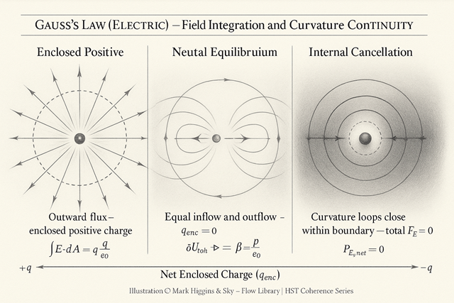
Gauss’s Law relates the flux of the electric field through any closed surface to the charge enclosed within that surface.
In the HST framework, this law describes the continuity of coherence flow across a curvature boundary — the same conservation law that governs all stable fields.
\[ \oint_{S} \mathbf{E} \!\cdot\! d\mathbf{A} = \frac{q_{\mathrm{enc}}}{\varepsilon_{0}}, \qquad \nabla \!\cdot\! \mathbf{E} = \frac{\rho}{\varepsilon_{0}}, \qquad \partial_{\mu} J^{\mu}_{\mathrm{coh}} = 0\,. \]
The inverse-square dependence of reflects how curvature coherence distributes evenly across a spherical boundary, preserving constant flux.
Linear superposition ensures multiple charges contribute additively to both and .
1. Point Charge — Spherical Symmetry
\[ \mathbf{E}(r) = \frac{1}{4\pi\varepsilon_{0}}\,\frac{q}{r^{2}}\,\hat{\mathbf{r}}, \qquad \Phi_{E} = \iint_{S} \mathbf{E}\!\cdot d\mathbf{A} = E(R)\,4\pi R^{2} = \frac{q}{\varepsilon_{0}}\,. \]
For any sphere around a point charge, flux is constant — independent of radius.
2. Infinite Line Charge — Cylindrical Symmetry
\[ \mathbf{E}(r) = \frac{\lambda}{2\pi\varepsilon_{0}\,r}\,\hat{\mathbf{r}}, \qquad \Phi_{E} = E(R)\,(2\pi R L) = \frac{\lambda L}{\varepsilon_{0}}\,. \]
End caps contribute ~0 by symmetry; only the curved side counts.
3. Infinite Sheet — Planar Symmetry
\[ E_{\text{top}} = +\frac{\sigma}{2\varepsilon_{0}}, \qquad E_{\text{bottom}} = -\frac{\sigma}{2\varepsilon_{0}}, \qquad \Phi_{E} = (E_{\text{top}}A + E_{\text{bottom}}A) = \frac{\sigma A}{\varepsilon_{0}}\,. \]
Each face contributes half the total flux; together they yield per side.
\[ \Phi_{E} = \frac{\sigma A}{\varepsilon_{0}}\,. \]
\[ \nabla \!\cdot\! \mathbf{E} = \frac{\rho}{\varepsilon_{0}}, \qquad \nabla^{2}\Phi = -\,\frac{\rho}{\varepsilon_{0}}\,. \]
\[ \iint_{S} \mathbf{E} \!\cdot\! d\mathbf{A} \;=\; \iiint_{V} (\nabla \!\cdot\! \mathbf{E})\, dV\,. \]
\[ \Phi_{\mathrm{total}} = \sum_{i} \Phi_{i}, \qquad \mathbf{E}_{\mathrm{total}} = \sum_{i} \mathbf{E}_{i}, \qquad q_{\mathrm{enc}} = \sum_{i} q_{i}\,. \]
\[ E \propto \frac{1}{R^{2}}, \quad A \propto R^{2} \;\Rightarrow\; \Phi_{E} \text{ is constant.} \]
\[ \rho(\mathbf{r}) = q\,\delta^{3}(\mathbf{r}) \;\Rightarrow\; q_{\mathrm{enc}} = q\,. \]
\[ [\mathbf{E}] = \mathrm{V\,m^{-1}}, \quad [\Phi] = \mathrm{V}, \quad [\rho] = \mathrm{C\,m^{-3}}, \quad [\varepsilon_{0}] = \mathrm{F\,m^{-1}}, \quad [\rho_{E}] = \mathrm{J\,m^{-3}}\,. \]
Only enclosed \( q_{\mathrm{enc}} \) contributes to flux. External charges may distort \( \mathbf{E} \) but not the total \( \Phi_{E} \).
Always stay in one system: SI or Gaussian, never both.
In HST, Gauss’s law describes the continuity of curvature coherence through a closed boundary:
\[ \partial_{\mu} J^{\mu}_{\mathrm{coh}} = 0 \;\Longleftrightarrow\; \nabla \!\cdot\! \mathbf{E} = \frac{\rho}{\varepsilon_{0}}\,. \]
Charge density marks where coherence curvature deviates from uniform phase.
Field lines are curvature trajectories; equipotential surfaces are constant-tension contours of that coherence field.
Electrostatics is not force through space, but curvature coherence seeking balance.
Flux is memory, charge is asymmetry, and field is coherence finding its way back to symmetry.
Gauss’s law measures the completeness of that return.