Chapter 21
Maxwell’s Unified Recursion
Field and Energy Systems
Author: Mark Anthony Higgins
Revised Date: 23 February 2026
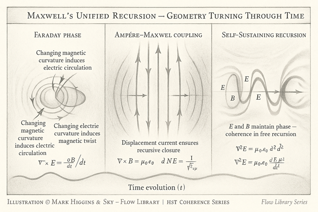
MaxwellsUnifiedRecursion reveals that the four classical equations of electromagnetism are not independent but iterative expressions of a single self-correcting law — coherence recursion.
Electric and magnetic fields are alternating aspects of the same curvature.
Each drives the other through time, and the displacement current term completes the feedback loop, ensuring coherence continuity even without charge motion.
In HST, Maxwell’s equations describe the recursion of coherence:
curvature generating phase, phase generating curvature — a perfectly closed feedback that manifests as light.
Maxwell’s unification is the mathematical realisation of dynamic coherence.
When curvature changes, it cannot vanish — it transforms into an orthogonal form that preserves total coherence.
This rotation of field alignment between E and B occurs with a fixed geometric ratio defined by the vacuum itself:
\[ c = \frac{1}{\sqrt{\varepsilon_{0}\mu_{0}}}\,. \]
Thus, light is not an entity travelling through empty space; it is pure coherence rotation moving at the natural recursion rate of the vacuum geometry.
The unified recursion consists of four interlinked conservation statements:
1. Gauss (Electric):
\[ \nabla \!\cdot\! \mathbf{E} = \frac{\rho}{\varepsilon_{0}}\,. \]
Boundary charge is a local curvature imbalance — the origin of phase tension.
2. Gauss (Magnetic):
\[ \nabla \!\cdot\! \mathbf{E} = \frac{\rho}{\varepsilon_{0}}\,. \]
Magnetic curvature is self-closed; coherence lines form continuous loops.
3. Faraday Induction:
∇×E=−∂t∂B.
Changing magnetic twist creates electric phase motion — coherence converting curvature into flow.
4. Ampère–Maxwell Coupling:
\[ \nabla \times \mathbf{B} = \mu_{0}\mathbf{J} + \mu_{0}\varepsilon_{0}\frac{\partial \mathbf{E}}{\partial t}\,. \]
Changing electric phase produces magnetic twist — coherence completing the rotation.
The result is a recursive field engine:
\[ \nabla^{2}\mathbf{E} = \mu_{0}\varepsilon_{0}\,\frac{\partial^{2}\mathbf{E}}{\partial t^{2}}, \qquad \nabla^{2}\mathbf{B} = \mu_{0}\varepsilon_{0}\,\frac{\partial^{2}\mathbf{B}}{\partial t^{2}}\,. \]
These are the wave equations of free coherence — geometry sustaining itself by perpetual phase exchange.
The recursion obeys the Poynting theorem:
\[ \frac{\partial u}{\partial t} + \nabla \!\cdot\! \mathbf{S} = -\,\mathbf{J}\!\cdot\!\mathbf{E}, \qquad u = \tfrac{1}{2}\!\left( \varepsilon_{0}|\mathbf{E}|^{2} + \tfrac{1}{\mu_{0}}|\mathbf{B}|^{2} \right), \qquad \mathbf{S} = \tfrac{1}{\mu_{0}}(\mathbf{E} \times \mathbf{B})\,. \]
Here \( u \) is the stored curvature energy density, and \( \mathbf{S} \) is the flow of coherence energy.
When \( \nabla\!\cdot\!\mathbf{S} = 0 \), coherence remains bound (standing field).
When \( \nabla\!\cdot\!\mathbf{S} > 0 \), coherence radiates outward as electromagnetic waves — geometry breathing freely.
\[ \mathbf{E} \xrightarrow{\;\partial_t\;} \mathbf{B} \xrightarrow{\;\partial_t\;} \mathbf{E}\,. \]
Each derivative step converts curvature phase into its orthogonal form, producing an oscillation.
One full cycle corresponds to a complete rotation of coherence in four-dimensional phase space — a photon’s heartbeat.
The displacement current \( \varepsilon_{0}\dfrac{\partial \mathbf{E}}{\partial t} \) is the phase continuity term that closes the recursion even when \( \mathbf{J} = 0 \). Without it, coherence would break at the boundary; with it, the field remains self-consistent everywhere.
Boundaries determine whether recursion remains closed or radiates outward:
Thus, radiation is not a separate phenomenon but open-boundary recursion — coherence released into global equilibrium.
| Classical description | Coherence interpretation |
|---|---|
|
Electric field
𝐸
|
Phase curvature (potential gradient)
|
|
Magnetic field
𝐵
|
Rotational curvature (spatial twist)
|
|
Displacement current
|
Time-phase continuity term \( \partial_{\mu} J^{\mu} = 0 \)
|
|
Poynting vector
𝑆
|
Flow of curvature coherence
|
|
Speed of light
𝑐
|
Recursion rate of vacuum coherence
|
|
Electromagnetic wave
|
Self-propagating curvature feedback
|
The “four Maxwell equations” are therefore four boundary views of a single recursive conservation law:
\[ \partial_{\mu} J^{\mu}_{\mathrm{coh}} = 0\,. \]
Maxwell’s system is the first complete expression of self-referential geometry — a law that not only describes motion but enforces its own continuity.
The fields we measure are the visible ripples of an invisible recursion:
coherence conserving itself by turning curvature through time.
The vacuum is not emptiness; it is equilibrium.
Electromagnetic fields are its oscillations — its memory in motion.
Light, therefore, is not transmitted energy, but recurring coherence made visible.
The speed of light is the speed of memory — the rate at which coherence rebalances itself.
Maxwell’s Unified Recursion completes the electromagnetic architecture of HST.
It shows that all fields, forces, and radiations are modes of recursive curvature balance — the universe continually realigning its coherence across space and time.
The same recursion pattern reappears in gravity, sound, plasma, and consciousness itself: a feedback engine where structure and motion are one.
When coherence turns, light emerges.
When light turns, geometry breathes.
And when geometry breathes, the universe endures.
Maxwell’s equations are the recursive heartbeat of coherence.
They do not describe fields acting on matter, but geometry remembering itself through rotation.
Every photon is a loop of coherence — curvature reciting its own name across time.