
Chapter 13
Correspondence Principle (Re-derived)

Meta-Principles of Coherence Physics
Author: Mark Anthony Higgins
© Mark Anthony Higgins 11 October 2025
Revised Date: 23 February 2026
Audio Overview
Flow Algebra
flow "CorrespondencePrinciple_ReDerived"

# ---------- STATES ----------
state:
  system.scale.λ_coh: float              # characteristic coherence wavelength
  system.scale.L: float                  # macroscopic system scale
  field.phase.Φ: float                   # mean coherence phase
  field.variance.ΔΦ: float               # phase dispersion
  curvature.tension.Σ: float             # boundary curvature tension density
  action.S: float                        # classical action functional
  action.quantum.Sħ: float               # quantised action (S / ħ)
  energy.E: float                        # system energy
  momentum.p: float                      # system momentum
  position.x: float                      # representative coordinate
  wavefunction.ψ: complex                # coherence amplitude
  probability.ρ: float                   # |ψ|²
  classical_limit: bool                  # indicator (true if coherence → continuum)
  correspondence.integrity: float        # 0..1; overlap between quantum and classical regimes
  hbar: float                            # Planck constant (6.626e-34 Js)
  time.t: float

# ---------- PARAMETERS ----------
params:
  hbar: 1.054e-34
  k_coh: float                            # curvature–coherence constant
  ΔΦ_threshold: 0.05                      # small-phase-dispersion threshold for classical limit
  dt: float

# ---------- INVARIANTS ----------
invariant:
  - quantisation condition:  S / params.hbar = 2πn  (closed coherence loop)
  - correspondence:  ⟨observable⟩_quantum → observable_classical  as  λ_coh / L → 0
  - field.phase.Φ evolves via Schrödinger:  iħ ∂ψ/∂t = Hψ
  - in high-coherence (ΔΦ ≪ 1), phase fronts align → Hamilton–Jacobi equation recovered
  - limit(ħ→0) ≡ limit(λ_coh / L → 0) : coherence oscillations average out
  - action continuity: δS = 0 holds in both classical and quantum frames (stationary coherence path)
  - correspondence.integrity = 1 − |⟨observable⟩_q − observable_c| / observable_c

# ---------- TRANSFORMS ----------
transform:

  initialise_system:
    do:
      system.scale.L = 1.0e-2           # macroscopic reference (m)
      system.scale.λ_coh = 1.0e-9       # nanometre-scale coherence
      field.variance.ΔΦ = 0.2
      correspondence.integrity = 0.9
      classical_limit = false
      wavefunction.ψ = exp(i*field.phase.Φ)
      probability.ρ = |wavefunction.ψ|^2
      time.t = 0

  compute_coherence_ratio:
    do:
      ratio = system.scale.λ_coh / system.scale.L
      if ratio << 1:
        classical_limit = true
      else:
        classical_limit = false

  evolve_phase:
    do:
      # Schrödinger → Hamilton–Jacobi correspondence
      field.phase.Φ += (energy.E - (momentum.p^2)/(2m)) * params.dt / params.hbar
      field.variance.ΔΦ = update_phase_variance(field.phase.Φ, params.k_coh)

  update_action:
    do:
      action.S = integrate_over_path(momentum.p, position.x)
      action.quantum.Sħ = action.S / params.hbar
      curvature.tension.Σ = params.k_coh * sin(field.phase.Φ)

  check_correspondence:
    do:
      if field.variance.ΔΦ < params.ΔΦ_threshold and classical_limit:
        correspondence.integrity = min(correspondence.integrity + 0.01, 1.0)
      elif field.variance.ΔΦ > 0.5:
        correspondence.integrity = max(correspondence.integrity - 0.05, 0.5)

  transition_mapping:
    do:
      # derive classical observables as averages over coherent microstates
      observable_quantum = ⟨ψ|Ô|ψ⟩
      observable_classical = time_average(observable_quantum, ΔΦ)
      correspondence.integrity = 1 - abs(observable_quantum - observable_classical)/max(observable_classical,1e-9)
      if correspondence.integrity > 0.98:
        mark("quantum_to_classical_bridge")

  tick:
    do:
      time.t += params.dt

# ---------- MONITORS ----------
monitor:
  coherence_ratio:
    observe: [system.scale.λ_coh, system.scale.L, classical_limit]
    report: "Shows when coherence wavelength is small compared to system scale — classical limit reached."

  phase_alignment:
    observe: [field.variance.ΔΦ, correspondence.integrity]
    report: "Tracks how phase dispersion determines overlap between quantum and classical observables."

  action_equivalence:
    observe: [action.S, action.quantum.Sħ]
    report: "Compares stationary action in classical and quantum regimes; equality confirms correspondence."

# ---------- NOTES (coherence view) ----------
note:
  - The classical limit arises not from ħ → 0 physically, but from **λ_coh / L → 0**, where coherence oscillations average into smooth curvature motion.
  - Quantum mechanics describes localised coherence oscillations (phase-quantised boundaries); classical mechanics describes averaged coherence (phase continuum).
  - The Schrödinger equation reduces to Hamilton–Jacobi when coherence phases align: ∂S/∂t + (∇S)²/2m + V = 0.
  - Every classical trajectory corresponds to the **mean path of many micro-coherence loops** — the ensemble phase average of HST’s boundary lattice.
  - Stationary action δS = 0 is the same condition as stationary coherence (δΦ = 0 modulo 2π).
  - Quantum uncertainty corresponds to finite boundary curvature; classical determinism arises when the curvature field flattens and coherence phases synchronise.
  - Thus, the Correspondence Principle is the **continuity of coherence**, not a limiting contradiction between two theories.
  - In perfect coherence (integrity = 1), the transition is seamless: quantum probabilities converge to classical predictability.

What this flow captures

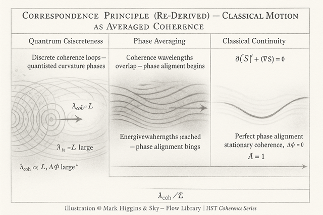
CorrespondencePrinciple_ReDerived reformulates the classical–quantum boundary not as a limit where Planck’s constant “goes to zero,” but as a coherence transition within the same geometric field.
In HST, both classical and quantum descriptions are approximations of a single, continuous structure — boundary coherence at different scales.

Quantum mechanics represents localised phase curvature where coherence loops are small and discrete.
Classical mechanics represents averaged curvature motion where those loops overlap so densely that their phase oscillations cancel, leaving a smooth trajectory.
The Correspondence Principle is therefore not a boundary between two worlds, but the self-averaging of coherence as system size increases.


Core intuition (HST view)

In standard physics, the Correspondence Principle demands that quantum results reduce to classical predictions in the macroscopic limit.

In HST, this happens because the system’s coherence wavelength λcoh\lambda_{\mathrm{coh}} becomes negligible compared to its macroscopic scale LL.
The ratio λcoh/L\lambda_{\mathrm{coh}} / L defines whether the system behaves as discrete (quantum) or continuous (classical).

When λcoh≪L\lambda_{\mathrm{coh}} \ll L, individual phase oscillations average out:

⟨observable⟩quantum​→observableclassical​.

At that point, interference fringes dissolve into continuity — coherence remains, but as an unresolvable background smoothness.
The laws of classical mechanics emerge as the large-scale limit of phase coherence, not as a separate regime.


Mathematical structure
Start with a Lagrangian density:

\[ \mathcal{L}(\phi,\,\partial_{\mu}\phi) \]

and define the quantum amplitude through the action SS:

\[ \psi = A\,e^{\,iS/\hbar}\,. \]

Inserting this into the Schrödinger equation:

\[ i\hbar\,\frac{\partial \psi}{\partial t} = H\psi\,. \]

and separating real and imaginary parts gives:

The continuity equation (probability current):

\[ \frac{\partial \rho}{\partial t} + \nabla \!\cdot\! (\rho\,\mathbf{v}) = 0\,. \]

The Hamilton–Jacobi equation (classical limit):

\[ \frac{\partial S}{\partial t} + \frac{(\nabla S)^2}{2m} + V = 0\,. \]

\[ \text{Thus, the quantum equation reduces to the classical one when phase coherence } \Phi \text{ varies smoothly — when internal oscillations average to a continuous curvature field.} \] \[ \text{The conventional limit } (\hbar \to 0) \text{ is equivalently expressed in HST as } \frac{\lambda_{\mathrm{coh}}}{L} \to 0\,. \]

Interpretation in coherence physics
ConceptConventional viewHST reinterpretation
ħ → 0 classical limit
Quantum behaviour
disappears
Coherence wavelength
becomes infinitesimal
— phases align
Deterministic motion
Classical certainty
Perfect phase coherence (ΔΦ → 0)
Probability wave
Quantum superposition
Finite curvature interference pattern
Trajectory
Path of a particle
Mean path of overlapping coherence loops
Uncertainty
Limitation of knowledge
Expression of finite boundary curvature
Action (S)
Minimises path integral
Stationary coherence
functional (δS = 0 ⇔ δΦ = 0 mod 2π)

In this framing, the action principle and phase stationarity are the same law written in different languages.
Both describe the geometry seeking coherence equilibrium.


Boundary coherence and determinism
  • When the coherence integrity Icoh=1I_{\mathrm{coh}} = 1: all phase fronts align; motion follows a single deterministic path — the classical trajectory.
  • When Icoh<1I_{\mathrm{coh}} < 1: phase dispersion introduces interference; probability amplitudes appear.
  • The transition is continuous: determinism is just perfect coherence, and quantum indeterminacy is finite curvature tension.

Every physical system lies somewhere along this continuum, with the macroscopic world simply operating at coherence scales where phase variation is imperceptible.


Energy and information continuity

HST resolves the classical–quantum duality by treating energy and information as two views of the same coherence current:

\[ J^{\mu}_{\mathrm{coh}} = \rho\,u^{\mu} \;\Rightarrow\; \partial_{\mu} J^{\mu}_{\mathrm{coh}} = 0\,. \]

When coherence is localised (quantum), this current exhibits interference; when coherence is global (classical), it smooths into an invariant flow.
The conservation of energy is thus equivalent to conservation of coherence — the persistence of stationary curvature phase through transformation.


Philosophical interpretation
  • Quantum mechanics is fine-grain coherence geometry.
    It reveals the structure of reality before averaging.
  • Classical mechanics is coarse-grain coherence geometry.
    It’s the macroscopic texture of the same fabric.
  • The Correspondence Principle is continuity of description.
    Not the replacement of one theory by another, but the realisation that both are slices of one coherence spectrum.

Significance

This re-derivation restores unity between the quantum and classical realms: both emerge from the same curvature logic, differing only by coherence resolution.
The limit is not in physics but in perception — the scale at which coherence fluctuations can or cannot be resolved.

Thus, HST transforms the Correspondence Principle from a statement of approximation into a statement of geometric continuity:

Classical motion is quantum coherence too large to notice.


In essence

The classical world is the shadow of perfect coherence; the quantum world its texture.
Both are phases of the same field — the geometry of continuity.


Kireth Research
38 Thorndale Croft, Wetwang, Driffield
East Riding of Yorkshire YO25 9XZ
Designed By