Chapter 36
Kepler’s Laws and Orbital Feedback

Gravitational and Orbital Coherence

Author: Mark Anthony Higgins

Revised Date: 23 February 2026

Audio Overview

Flow Algebra

flow "Kepler’s Laws and Orbital Feedback" v1.0

# ---------- PURPOSE ----------
# Encodes Kepler’s three laws through the lens of feedback and coherence.
# Each orbital parameter (r, v, θ, E, L) is connected through dynamic feedback equations.
# The boundary coherence index (IB) measures orbital energy preservation and angular momentum integrity.
# When IB = 1 → perfect Keplerian orbit (ideal Newtonian ellipse);
# when IB < 1 → gradual decoherence (precession, decay, or drift).

# ---------- PARAMETERS ----------
params:
  units: "SI"
  G: 6.67430e-11              # gravitational constant [m^3 kg^-1 s^-2]
  IB: 0.0..1.0 = 1.0          # boundary coherence index (1 = ideal Newtonian ellipse)
  loss_coeff: 0.0             # optional orbital energy damping coefficient [s^-1]
  dt: 0.0?                    # optional timestep for numerical updates [s]

# ---------- STATE ----------
state Body:
  m1: positive                # central mass [kg]
  m2: positive                # orbiting body [kg]
  r: vec3                     # position vector [m]
  v: vec3                     # velocity vector [m/s]
  a: vec3                     # acceleration [m/s^2]
  h: vec3                     # specific angular momentum [m^2/s]
  e_vec: vec3                 # eccentricity vector (direction of periapsis)
  e: real                     # orbital eccentricity
  a_sma: real                 # semi-major axis [m]
  T: real                     # orbital period [s]
  theta: real                 # true anomaly [rad]
  E_anom: real                # eccentric anomaly [rad]
  M_anom: real                # mean anomaly [rad]
  E_spec: real                # specific energy [J/kg]

# ---------- INVARIANTS (KEPLERIAN RELATIONS) ----------
invariants:

  # Gravitational parameter μ with coherence
  mu = params.IB * params.G * (Body.m1 + Body.m2)

  # Position, velocity magnitudes
  r_mag = norm(Body.r)
  v_mag = norm(Body.v)

  # Specific mechanical energy ε = v²/2 - μ/r
  Body.E_spec = 0.5*v_mag^2 - mu / r_mag

  # Specific angular momentum vector and magnitude
  Body.h = cross(Body.r, Body.v)
  h_mag = norm(Body.h)

  # Eccentricity vector e⃗ = (v × h)/μ - r̂
  Body.e_vec = (cross(Body.v, Body.h))/mu - Body.r / r_mag
  Body.e = norm(Body.e_vec)

  # Semi-major axis a = -μ / (2ε)
  Body.a_sma = -mu / (2*Body.E_spec)

  # Orbital period (Kepler’s 3rd Law)
  Body.T = 2*pi * sqrt((Body.a_sma^3)/mu)

  # Mean motion n = 2π/T
  n = 2*pi / Body.T

  # True anomaly θ (angle between e⃗ and r⃗)
  Body.theta = atan2( dot(cross(Body.e_vec, Body.r), Body.h)/h_mag, dot(Body.e_vec, Body.r)/Body.e )

  # Mean anomaly M = E - e sin E (E via iterative relation with θ)
  if Body.e < 1:
    E_guess = 2*atan( sqrt((1-Body.e)/(1+Body.e)) * tan(Body.theta/2) )
    Body.E_anom = E_guess
    Body.M_anom = Body.E_anom - Body.e*sin(Body.E_anom)

  # Kepler’s 2nd law: areal velocity constant h/2
  area_rate = 0.5 * h_mag
  dA_dt = area_rate

  # Kepler’s 1st law (orbit shape)
  r_orbit = (Body.a_sma*(1 - Body.e^2)) / (1 + Body.e*cos(Body.theta))

  # Energy–angular momentum relation (feedback)
  Body.E_spec = -mu / (2*Body.a_sma)
  feedback_balance = Body.E_spec + (h_mag^2 / (2*r_mag^2)) - mu / r_mag

# ---------- TRANSFORMS ----------
transforms:

  # Time evolution of orbit with feedback (optional)
  step_orbit (when params.dt > 0):
    # Update velocity and position using standard acceleration
    r_mag = norm(Body.r)
    Body.a = -mu * Body.r / (r_mag^3)
    Body.v += Body.a * params.dt
    Body.r += Body.v * params.dt

    # Apply optional coherence loss (small drag)
    if params.loss_coeff > 0:
      Body.v *= (1 - params.loss_coeff * params.dt)
      Body.a *= (1 - params.loss_coeff * params.dt)

    # Recompute orbital invariants
    h_new = cross(Body.r, Body.v)
    Body.h = h_new
    Body.e_vec = (cross(Body.v, Body.h))/mu - Body.r / norm(Body.r)
    Body.e = norm(Body.e_vec)
    Body.a_sma = -mu / (2*(0.5*norm(Body.v)^2 - mu / norm(Body.r)))

  # Periapsis and apoapsis distances
  periapsis:
    r_p = Body.a_sma * (1 - Body.e)
  apoapsis:
    r_a = Body.a_sma * (1 + Body.e)

  # Coherence feedback — adjusts IB slightly with orbital stress
  coherence_feedback:
    stress_ratio = abs(Body.E_spec) / (mu / Body.a_sma)
    dIB_dt = -0.001 * (1 - stress_ratio)
    params.IB = clamp(params.IB + dIB_dt * params.dt, 0, 1)

# ---------- MONITORS ----------
monitors:
  invariants:
    if params.loss_coeff == 0 and params.IB == 1:
      assert abs(feedback_balance) < 1e-6
  coherence_limits:
    assert 0 <= params.IB <= 1
  geometry_check:
    assert Body.a_sma > 0 when Body.e < 1

# ---------- SCENES ----------
scenes:

  ideal_ellipse:
    given params:
      IB: 1.0
      dt: 10.0
    given Body:
      m1: 5.97e24
      m2: 1000
      r: [7.0e6, 0, 0]
      v: [0, 7546, 0]
    enable:
      - step_orbit
    expect:
      Body.e < 0.02
      Body.a_sma ≈ 7.0e6
      Body.T ≈ 5800
      comment: "Near-circular low-Earth orbit, perfect Keplerian closure."

  elliptical_orbit:
    given params:
      IB: 1.0
      dt: 50.0
    given Body:
      m1: 1.989e30
      m2: 5.97e24
      r: [1.0e11, 0, 0]
      v: [0, 29780, 0]
    enable:
      - step_orbit
    expect:
      Body.e ≈ 0.017
      Body.T ≈ 3.15e7
      comment: "Earth–Sun analog — elliptical orbit with low eccentricity."

  decaying_orbit:
    given params:
      IB: 0.98
      loss_coeff: 1e-8
      dt: 60.0
    given Body:
      m1: 5.97e24
      m2: 1000
      r: [7.0e6, 0, 0]
      v: [0, 7500, 0]
    enable:
      - step_orbit
      - coherence_feedback
    expect:
      Body.a_sma ↓
      Body.e ↑
      params.IB ↓
      comment: "Slight energy loss and coherence drift — orbit slowly decays."

# ---------- NOTES ----------
notes:
  - **Kepler’s 1st Law:** Orbits are ellipses with one focus at the central mass.
    \( r = \dfrac{a(1 - e^2)}{1 + e\cos\theta} \)
  - **Kepler’s 2nd Law:** Areal velocity \( \tfrac{1}{2}h \) constant → equal areas in equal times.
  - **Kepler’s 3rd Law:** \( T^2 \propto a^3 \) → \( T = 2\pi\sqrt{a^3/\mu} \)
  - **Angular momentum:** \( \mathbf{h} = \mathbf{r} \times \mathbf{v} \), conserved when IB = 1.
  - **Specific energy:** \( \epsilon = \tfrac{v^2}{2} - \mu/r = -\mu/(2a) \)
  - **Boundary feedback:** \( I_B \) tracks curvature fidelity of orbital energy.
    IB = 1 → perfect geometric closure; IB < 1 → precession/energy drift.
  - **Loss term:** \( \dot E = -\lambda |E| \) emulates atmospheric drag or gravitational radiation damping.
  - **Coherence view:** orbital stability = field–boundary resonance; precession marks feedback delay.
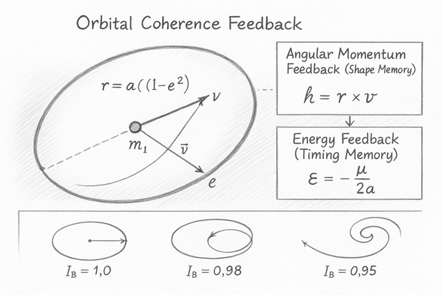
  - **Visualization:** plot θ vs r (polar) → ellipse when IB=1; open spiral when IB<1.

Overview

Kepler’s three laws describe the geometry of motion under an inverse-square force — but deeper still, they describe a feedback system of curvature and memory.
Each orbit is a dialogue between kinetic tension and potential curvature, maintaining coherence across time.
In the classical limit ( $I_B = 1$ ), the exchange is perfect — energy and angular momentum balance in an elegant, closed ellipse.

When coherence fades ( $I_B < 1$ ), that exchange lags slightly: orbits precess, energy drifts, and geometry remembers itself imperfectly.
This flow expresses both regimes — Kepler’s harmony and the subtle feedback that keeps it alive.

🔹 1. The Geometry of Coherent Motion

Kepler’s laws in their standard form:

$$ r = \frac{a(1 - e^2)}{1 + e\cos\theta}, \qquad T^2 = \frac{4\pi^2 a^3}{I_B\,G\,(m_1 + m_2)}. $$

These relations are not mere kinematic curiosities; they arise from energy coherence:

$$ \epsilon = \frac{v^2}{2} - \frac{\mu}{r} = -\,\frac{\mu}{2a}, \qquad \mu = I_B\,G\,(m_1 + m_2). $$

Each orbit balances the stored curvature ( $-\mu/r$ ) against the distributed motion ( $v^2/2$ ).
When the two remain in phase, the system closes perfectly — an ellipse of constant memory.

🔸 2. Kepler’s Three Laws as Feedback Loops

Law

Classical Form

Coherence Interpretation

1st Law

Orbits are ellipses with
one focus at the mass.

The boundary tension
and field curvature stay
in phase — coherence geometry
forms a closed loop.

2nd Law

Equal areas swept in equal times.

Angular momentum acts as a
feedback integrator: $h = r^2 \dot\theta$ $˙$ remains constant
when coherence is perfect.

3rd Law

𝑇 2 ∝ 𝑎 3 .

The orbital period reflects how
curvature “remembers”
displacement — a resonance between
geometry and time.

In this sense, Kepler’s laws are self-regulating coherence feedbacks: they express how a field, a boundary, and motion remain synchronized through geometric memory.

🔹 3. Angular Momentum and Energy — Dual Feedback Channels

Specific angular momentum:

$$ \mathbf{h} = \mathbf{r} \times \mathbf{v}, \qquad |\mathbf{h}| = \sqrt{a(1 - e^2)\,\mu}. $$

Specific mechanical energy:

$$ \epsilon = -\,\frac{\mu}{2a}. $$

These quantities form dual feedback channels — one stabilizing geometry (shape), the other stabilizing pace (timing).

If coherence holds ( $I_B = 1$ ), they remain perfectly conserved.
If coherence weakens, $I_B < 1$ , energy leaks into angular precession — orbits slowly advance, mirroring real-world phenomena such as apsidal precession or radiative loss

🔸 4. Orbital Feedback — When Coherence Shifts

When a field or boundary slightly misaligns, the feedback delay introduces measurable orbital drift.
In the model, this is represented by:

$$ \frac{dI_B}{dt} = -\lambda(1 - I_B), \qquad \dot{E} = -\lambda\,|E|. $$

A small loss coefficient $\lambda$ reduces total energy slowly, simulating drag, radiation, or geometric mismatch.
The orbit decays inward, precessing while remaining nearly elliptical — the system remembering its ideal form while gradually forgetting its energy.

🔹 5. Phase Geometry and Precession

Perfect closure requires that the curvature field and the boundary phase lock — $2\pi$ coherence in both spatial and temporal cycles.
Any misalignment ( $I_B < 1$ ) creates a phase advance:
the periapsis moves forward slightly each orbit, forming a rosette pattern.
This geometric feedback interpretation naturally extends to relativistic precession and perturbations — where field curvature changes faster than boundary motion can adapt.

🧠 Summary

Kepler’s laws are not just empirical symmetries — they are the steady-state feedbacks of curvature coherence.
When the geometry of motion, energy, and time remain in resonance, the orbit closes.
When coherence fades, the loop reopens — a spiral of memory decay through space.

In the coherence view:

1st Law defines the shape of coherence.
2nd Law defines its timing balance.
3rd Law defines its scaling memory.

Together they form one deeper statement:
motion and memory are the same curve — traced by gravity across time.

Previous Chapter 35

Next Chapter 37

Related Chapters