
Chapter 30
Equipartition and Energy Topology

Thermal and Entropic Flows
Author: Mark Anthony Higgins
© Mark Anthony Higgins 11 October 2025
Revised Date: 23 February 2026
Audio Overview
Flow Algebra
flow "Equipartition and Energy Topology" v1.0

# ---------- PURPOSE ----------
# Unifies the equipartition theorem with a topology-of-modes view.
# Each quadratic degree of freedom (DOF) contributes (1/2) k_B T when active.
# A mode-graph (energy topology) governs which DOFs are available and how coherence (IB) and coupling shape U(T) and C_V(T).
# Handles classical limit, low-T freeze-out, partial activation (vibrations/rotations), and coherence losses.

# ---------- PARAMETERS ----------
params:
  units: "SI"
  k_B: 1.380649e-23          # Boltzmann constant [J/K]
  N: positive                # number of particles (or moles*NA if you prefer to absorb NA into N)
  T: positive                # temperature [K]
  # Topology + activation controls
  include_quantum_freezeout: true
  include_coupling_losses:   true
  mix_uniform_when_incoherent: true
  # Default smoothness for activation (sigmoid width)
  w_T: 0.15                  # fractional width for activation sigmoid (relative to T*)
  # Optional gas constants if you want molar outputs (set N = n*NA if not using these)
  R: 8.314462618             # [J/(mol·K)] for convenience

# ---------- STATE ----------
# Mode j is a "site" in the energy topology graph.
# a_j = # of quadratic terms contributed by the mode (1 for x^2-only, 2 for q & p of a harmonic mode, etc.)
state ModeGraph:
  mode_id[]: str
  a_j[]: positive           # quadratic multiplicity per mode (1, 2, …)
  T_star[]: positive        # characteristic activation temperature for the mode [K]
  IB_j[]: 0.0..1.0          # coherence of mode boundary (1 = fully coherent)
  coup_loss_j[]: 0.0..1.0   # fractional loss from topological coupling/damping (0 = no loss)
  weight_j[]: positive=1.0  # optional weighting for degeneracy/multiplicity
  # Topology connectivity (optional, for advanced coupling shaping)
  edges[][2]: int?          # pairs of (i, k) indices indicating coupled modes (optional)

state Thermo:
  U:   real                 # internal energy [J]
  Cv:  real                 # heat capacity at constant volume [J/K]
  f_eff: real               # effective # of quadratic DOFs per particle
  gamma_note: str?          # optional note if used for ideal-gas gamma calculation

# ---------- HELPERS ----------
transforms:
  # Smooth activation function s_j(T): 0 (frozen) -> 1 (classically active)
  activation_sj:
    # Dimensionless temperature ratio and smoothness
    tau_j = params.T / max(ModeGraph.T_star, 1e-9)
    # logistic with width params.w_T around T_star
    s_raw = 1 / (1 + exp(-(tau_j - 1) / max(params.w_T, 1e-6)))
    # coherence + coupling shaping
    if params.include_coupling_losses:
      s_loss = max(0, 1 - ModeGraph.coup_loss_j)
    else:
      s_loss = 1
    # incoherence blending (toward uniform sharing that carries less structured energy)
    if params.mix_uniform_when_incoherent:
      s_coh = ModeGraph.IB_j * s_raw + (1 - ModeGraph.IB_j) * 0.5 * s_raw
    else:
      s_coh = ModeGraph.IB_j * s_raw
    s_j = clamp(s_coh * s_loss, 0, 1)

  # Optional quantum freeze-out refinement (Debye-/Einstein-like heuristic for harmonic modes)
  quantum_freezeout_factor:
    if params.include_quantum_freezeout:
      # crude Einstein factor: f_Q ~ (x^2 e^x)/(e^x - 1)^2 with x = T_star/T
      x = max(ModeGraph.T_star / max(params.T, 1e-9), 1e-9)
      f_Q = (x*x * exp(x)) / pow(exp(x) - 1, 2)
    else:
      f_Q = 1

# ---------- INVARIANTS (EQUIPARTITION + TOPOLOGY) ----------
# Classical equipartition: each quadratic DOF contributes (1/2) k_B T to U when active.
# Here: activation state s_j(T, IB, coupling) ∈ [0,1] scales the contribution; a_j counts quadratic terms.
invariants:
  # Per-mode contribution factor (including quantum freezeout heuristic)
  phi_j = activation_sj.s_j * quantum_freezeout_factor.f_Q

  # Effective DOFs per particle:
  # f_eff = Σ_j (a_j * weight_j * phi_j)
  Thermo.f_eff = sum(ModeGraph.a_j * ModeGraph.weight_j * phi_j)

  # Internal energy (per particle × N):
  # U = (1/2) k_B T * N * f_eff
  Thermo.U = 0.5 * params.k_B * params.T * params.N * Thermo.f_eff

  # Heat capacity at constant volume:
  # C_V = dU/dT ≈ (1/2) k_B N [ f_eff + T * d(f_eff)/dT ]
  # We provide the differential form; engines can compute numerically if needed.
  d_f_eff_dT = d/dT (Thermo.f_eff)           # symbolic; evaluate via autodiff or numeric step
  Thermo.Cv  = 0.5 * params.k_B * params.N * (Thermo.f_eff + params.T * d_f_eff_dT)

# ---------- MONITORS ----------
monitors:
  classical_high_T_limit:
    # As T >> T_star for all modes and IB_j→1, phi_j→1
    # Then f_eff → Σ a_j * weight_j, and C_V → (1/2) k_B N Σ a_j weight_j
    assert Thermo.f_eff >= 0
  low_T_freezeout:
    # As T → 0, phi_j → 0 (for vibrational/rotational modes with finite T*)
    assert Thermo.U >= 0
  coherence_bounds:
    assert all(0 <= ModeGraph.IB_j <= 1)
    assert all(0 <= ModeGraph.coup_loss_j <= 1)

# ---------- SCENES ----------
scenes:

  # Monoatomic ideal gas (translational only: 3 quadratic DOFs per particle → 3/2 k_B T)
  monatomic_gas:
    given params:
      T: 300
      N: 1.0                # per particle; set N = n*NA for molar
    given ModeGraph:
      mode_id:   ["Tx","Ty","Tz"]
      a_j:       [1, 1, 1]   # each translational axis contributes 1 quadratic term (KE = 1/2 m v^2 per axis)
      T_star:    [1, 1, 1]   # effectively always active
      IB_j:      [1, 1, 1]
      coup_loss_j:[0, 0, 0]
      weight_j:  [1, 1, 1]
    expect:
      Thermo.f_eff ≈ 3
      Thermo.U     ≈ 1.5 * params.k_B * params.T * params.N

  # Diatomic gas (3 trans + 2 rot active at room T; vib activates at higher T)
  diatomic_gas:
    given params:
      T: 300
      N: 1.0
      include_quantum_freezeout: true
    given ModeGraph:
      mode_id:   ["Tx","Ty","Tz","R1","R2","Vib_q","Vib_p"]
      a_j:       [1,1,1, 1,1, 1,1]    # harmonic vibration has q & p → two quadratic terms
      T_star:    [1,1,1, 150,150, 2000,2000]  # rot activates ~150K; vib ~2000K (example scales)
      IB_j:      [1,1,1, 0.95,0.95, 0.9,0.9]
      coup_loss_j:[0,0,0, 0.05,0.05, 0.1,0.1]
      weight_j:  [1,1,1, 1,1, 1,1]
    expect (qualitative at 300 K):
      # 3 trans fully active, 2 rot largely active, vib mostly frozen → f_eff ≈ ~5
      Thermo.f_eff ≈ 5 ± 0.2
      Thermo.U     ≈ 0.5 * k_B * T * N * f_eff   # ~ (5/2) k_B T per particle

  # Vibrational turn-on (raise T to see C_V peak as modes activate)
  vib_turn_on_sweep:
    sweep T: [200, 400, 800, 1200, 2000, 3000]
    base_scene: diatomic_gas
    observe:
      - Thermo.Cv   # should rise as vib modes activate, then level toward classical limit of 7 DOFs (3 trans + 2 rot + 2 vib)

  # Coherence degradation (topology losses reduce effective activation)
  coherence_loss_demo:
    given params:
      T: 600
      N: 1.0
    given ModeGraph:
      mode_id:   ["Tx","Ty","Tz","R1","R2","Vib_q","Vib_p"]
      a_j:       [1,1,1, 1,1, 1,1]
      T_star:    [1,1,1, 150,150, 800,800]
      IB_j:      [0.9,0.9,0.9, 0.8,0.8, 0.6,0.6]
      coup_loss_j:[0.05,0.05,0.05, 0.1,0.1, 0.2,0.2]
      weight_j:  [1,1,1, 1,1, 1,1]
    expect:
      Thermo.f_eff < classical_high_T_limit_of(Σ a_j)
      Thermo.Cv suppressed vs. coherent case
      note: "Lower IB and higher coupling loss flatten C_V(T) and reduce U."

# ---------- NOTES ----------
notes:
  - Equipartition (classical): each quadratic DOF contributes (1/2) k_B T to U.
  - Energy topology: the system’s DOFs form a graph of modes; activation, coherence (IB), and coupling losses determine which modes contribute.
  - Low-T freeze-out: modes with T* >> T are inactive (phi_j ≈ 0), shrinking f_eff and C_V.
  - High-T classical limit: phi_j → 1, so f_eff → Σ a_j weight_j and C_V → (1/2) k_B N Σ a_j weight_j.
  - Vibrations typically contribute two quadratics per normal mode (q & p) → add k_B T per mode when fully active.
  - Rotations in linear molecules: two rotational DOFs active above a characteristic T*, third for non-linear molecules.
  - Coherence IB_j maps structured energy retention; coupling losses capture topological damping/anharmonic leakage.
  - For molar quantities, set N = n·N_A or simply divide results by N and multiply by R where convenient: C_V,molar ≈ (1/2) R Σ a_j weight_j in classical limit.
Overview

The equipartition theorem tells us that each independent quadratic mode in a system contributes an average energy of 12kBT\tfrac{1}{2}k_B T.

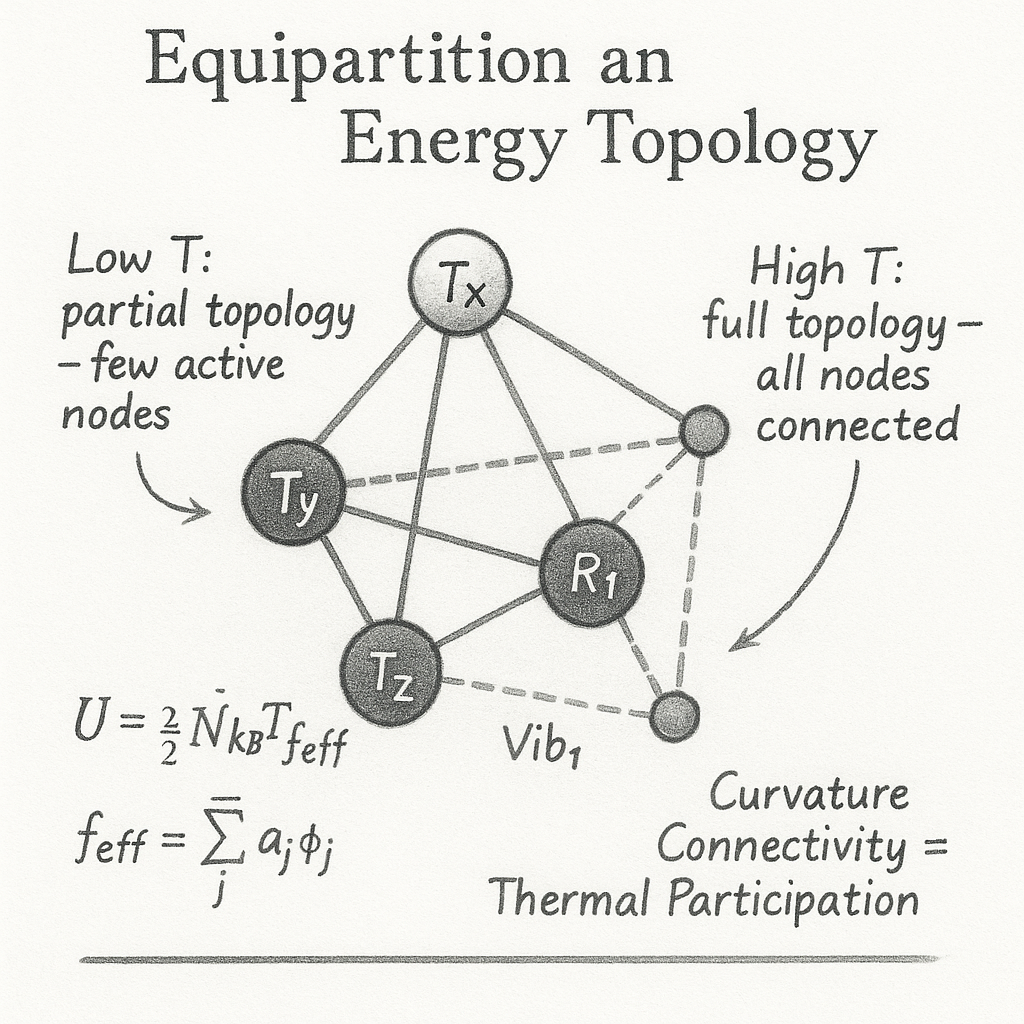
In Flow Algebra, this simple rule expands into a topology of energy modes — a map of how each degree of freedom (DOF) becomes active, coherent, or suppressed depending on its characteristic temperature, coupling, and coherence boundary IBI_B.

The structure of the system itself becomes a graph of modes, each with its own activation profile and curvature connection to others.


🔹 1. Core Principle — Distributed Thermal Activation

For every quadratic mode jj,

$$ \langle E_j \rangle = \frac{1}{2}\, k_B T\, \phi_j(T, I_B). $$

where the activation function ϕj∈[0,1]\phi_j \in [0,1] encodes the mode’s thermal accessibility and coherence:

$$ \phi_j = I_B\, s\!\left(\frac{T}{T^*}\right)\! (1 - \text{loss}_j). $$

with T∗T^* as the mode’s characteristic activation temperature and ss as a smooth logistic switch that transitions from frozen (00) to fully active (11).

At low TT, ϕj→0\phi_j \to 0: the mode is topologically isolated; at high TT, ϕj→1\phi_j \to 1: it joins the thermal manifold.


🧩 2. Energy Topology — A Graph of Modes

Each system’s internal structure can be represented as a mode graph:

  • Nodes represent active energy wells or oscillatory coordinates (translation, rotation, vibration).
  • Edges represent coupling or coherence channels between modes.
  • Each node carries a boundary coherence index IB,jI_{B,j} and a coupling loss λj\lambda_j, determining how strongly it participates in equipartition.

The effective number of active quadratic terms becomes:

$$ f_{\mathrm{eff}} = \sum_j a_j\, w_j\, \phi_j. $$

and thus,

$$ U = \frac{1}{2} N k_B T\, f_{\mathrm{eff}}, \qquad C_V = \frac{1}{2} N k_B \!\left( f_{\mathrm{eff}} + T\, \frac{d f_{\mathrm{eff}}}{dT} \right). $$

As coherence degrades (IB<1I_B < 1) or coupling losses rise, fefff_{\mathrm{eff}} drops — meaning not all energy modes share equally in the thermal balance.
Topology replaces simplicity with structure.


🧮 3. From Classical to Quantum Behaviour

At very low temperatures, quantum effects freeze out higher-energy modes, producing a selective topology of active degrees of freedom.
In the limit T≪T∗T \ll T^*,

$$ \phi_j \approx \exp\!\left(-\frac{T^*}{T}\right). $$

and the system retains only the modes with accessible energy curvature.
This transition naturally explains why heat capacity falls at cryogenic temperatures — the graph of available modes contracts.

At high temperatures, all modes fully engage:

$$ \lim_{T \to \infty} \phi_j = 1. $$

and the classical result re-emerges:

$$ U = \frac{1}{2} N k_B T \sum_j a_j, \qquad C_V = \frac{1}{2} N k_B \sum_j a_j. $$

The system becomes topologically complete — every curvature channel active and evenly sharing energy.


🌐 4. Coherence and Coupling — The Hidden Structure of Heat

Coherence IBI_B and coupling loss λj\lambda_j describe how real materials deviate from ideal equipartition:

  • High IBI_B: energy stored as stable, resonant curvature (elastic, reversible).
  • Low IBI_B: partial decoherence; energy scatters between boundaries or dissipates as phonon noise.
  • High λj\lambda_j: coupling loss between modes (anharmonicity, friction).
    Together, they form the energy topology of the system — a structured map of coherence flow between degrees of freedom.

From this perspective, equipartition is not simply statistical:
it is the self-organization of curvature across a field of interacting oscillators.
Temperature measures not just average kinetic energy, but the density of coherent participation in that topology.


🔭 5. Practical Interpretation
Temperature RegimeDominant ModesBehaviourCoherence Picture

T≪T∗

Translational only

Low \( C_V \) (frozen rotations/vibrations)

Partial topology
minimal connectivity

T∼T∗
Rotations activate
\( C_V \) rises smoothly
Network expansion
new curvature links
T≫T∗
Vibrations active

\( C_V \to \tfrac{7}{2} R \; \text{(for a diatomic gas)} \)

Fully coherent
network of modes

🧠 Summary

Equipartition is not a rule of arithmetic; it is a geometry of sharing.
Each degree of freedom is a doorway in the energy topology of a system.
As temperature rises, coherence opens more doors; as coupling or quantum limits close them, topology contracts.
In the HST framework, temperature measures not the chaos of motion but the completeness of boundary participation —
the extent to which the system’s internal geometry has awakened to coherence.


Kireth Research
38 Thorndale Croft, Wetwang, Driffield
East Riding of Yorkshire YO25 9XZ
Designed By