Chapter 19
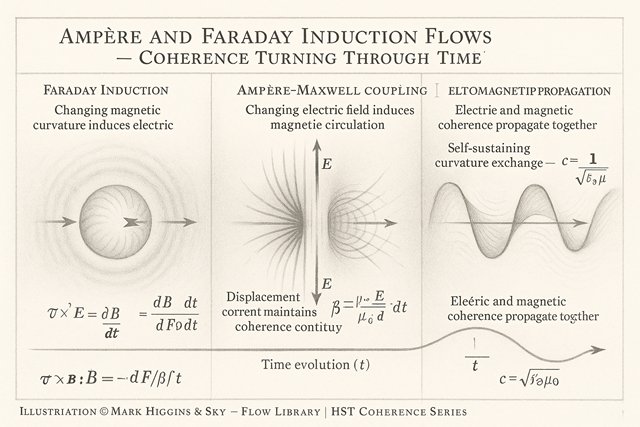
Ampère and Faraday Induction Flows

Flow Algebra

flow "Ampere_Faraday_InductionFlows"

# ---------- STATES ----------
state:
  field.E: vec[float,3]                  # electric field (V/m)
  field.B: vec[float,3]                  # magnetic flux density (T)
  current.density.J: vec[float,3]        # current density (A/m^2)
  displacement.current.Jd: vec[float,3]  # displacement current density (A/m^2)
  charge.density.ρ: float                # charge density (C/m^3)
  permittivity.ε0: float                 # permittivity of free space (F/m)
  permeability.μ0: float                 # permeability of free space (H/m)
  curl.E: vec[float,3]                   # ∇×E
  curl.B: vec[float,3]                   # ∇×B
  dE_dt: vec[float,3]                    # ∂E/∂t
  dB_dt: vec[float,3]                    # ∂B/∂t
  loop.C: curve                          # closed integration path
  surface.S: surface                     # surface bounded by C
  emf.ℰ: float                           # electromotive force (V)
  magnetic.flux.ΦB: float                # magnetic flux through S (Wb)
  circulation.B: float                   # ∮ B·dl (T·m)
  coherence.current.Jcohμ: vec[float,4]  # coherence flux analogue
  boundary.integrity: float              # 0..1, coherence continuity
  energy.density.ρE: float               # electric energy density (J/m^3)
  energy.density.ρB: float               # magnetic energy density (J/m^3)
  poynting.vector.S: vec[float,3]        # energy flux (W/m^2)
  time.t: float

# ---------- PARAMETERS ----------
params:
  ε0: 8.8541878128e-12
  μ0: 4π×10^-7
  c: 1/√(ε0μ0)
  dt: float
  k_coh: float

# ---------- INVARIANTS ----------
invariant:
  - Faraday’s law (differential): ∇×E = -∂B/∂t
  - Ampère–Maxwell law: ∇×B = μ0 J + μ0ε0 ∂E/∂t
  - Integral forms:
      ∮_C E·dl = - dΦB/dt
      ∮_C B·dl = μ0 I_enc + μ0ε0 dΦE/dt
  - Field energy densities:
      ρE = ½ ε0 |E|²,   ρB = ½ (1/μ0) |B|²
  - Energy continuity: ∂u/∂t + ∇·S = -J·E
      where S = (1/μ0)(E×B)
  - Coherence equivalence: ∂μ Jcoh^μ = 0 ↔ coupled field induction equilibrium
  - boundary.integrity = 1 for perfect coupling, <1 for dissipative or radiative loss

# ---------- TRANSFORMS ----------
transform:

  initialise_field:
    do:
      field.E = [0,0,0]
      field.B = [0,0,1e-3]
      current.density.J = [0,0,0]
      displacement.current.Jd = [0,0,0]
      charge.density.ρ = 0
      boundary.integrity = 0.995
      time.t = 0

  compute_faraday_induction:
    do:
      # Magnetic flux change induces electric circulation
      magnetic.flux.ΦB = surface_integral(field.B, surface.S)
      emf.ℰ = - d(magnetic.flux.ΦB)/dt
      curl.E = - partial_derivative(field.B, time)
      field.E += curl.E * params.dt
      update_coherence(current="inductive")

  compute_ampere_maxwell:
    do:
      # Electric change induces magnetic circulation
      displacement.current.Jd = params.ε0 * partial_derivative(field.E, time)
      curl.B = params.μ0 * (current.density.J + displacement.current.Jd)
      field.B += curl.B * params.dt
      update_coherence(current="displacement")

  update_energy_balance:
    do:
      energy.density.ρE = 0.5 * params.ε0 * |field.E|²
      energy.density.ρB = 0.5 * (1/params.μ0) * |field.B|²
      poynting.vector.S = (1/params.μ0) * cross(field.E, field.B)
      boundary.integrity -= small_radiative_loss(poynting.vector.S)

  update_coherence:
    do:
      coherence.current.Jcohμ = [energy.density.ρE + energy.density.ρB, poynting.vector.S]
      assert divergence(coherence.current.Jcohμ) ≈ 0
      if boundary.integrity < 0.98:
        mark("radiative_drift")

  tick:
    do:
      time.t += params.dt

# ---------- MONITORS ----------
monitor:
  induction_balance:
    observe: [curl.E, dB_dt]
    report: "Faraday induction: ∇×E = -∂B/∂t (coherence rotation in time)."

  ampere_balance:
    observe: [curl.B, current.density.J, displacement.current.Jd]
    report: "Ampère–Maxwell coupling: magnetic circulation sustained by conduction + displacement current."

  energy_flow:
    observe: [energy.density.ρE, energy.density.ρB, poynting.vector.S]
    report: "Tracks conversion between electric and magnetic coherence; ∂u/∂t + ∇·S = -J·E."

  boundary_health:
    observe: [boundary.integrity]
    report: "Boundary integrity near 1 implies reversible induction; loss marks radiative leakage."

# ---------- NOTES (coherence view) ----------
note:
  - Faraday’s law: changing magnetic coherence (curvature twist) induces electric phase circulation — ∇×E = -∂B/∂t.
  - Ampère–Maxwell law: changing electric curvature induces magnetic alignment — ∇×B = μ0J + μ0ε0∂E/∂t.
  - Both are two halves of the same coherence rotation: electric ↔ magnetic, potential ↔ curvature.
  - Displacement current (ε0 ∂E/∂t) ensures coherence continuity even without charge flow; it is the geometric memory of electric phase motion.
  - The Poynting vector S = (1/μ0)(E×B) expresses the flux of coherence energy — curvature tension in motion.
  - Radiation occurs when boundary integrity < 1 and coherence decouples into free waves.
  - In HST, Maxwell’s equations describe curvature feedback loops maintaining coherence between boundary phase (E) and boundary twist (B).
  - Static limits recover Gauss (electric) and Coulomb flow; dynamic coupling yields electromagnetic waves — pure curvature coherence in transit.

What this flow captures

Core intuition (HST view)

Mathematical structure

Ampère–Maxwell Law:

Energy conservation (Poynting theorem):

Interpretation in coherence physics

Boundary coherence and displacement

Energy and coherence flux

Unified geometric interpretation

• E: curvature phase gradient (potential flow).
• B: curvature twist (rotational coherence).
• Ampère + Faraday: orthogonal transformations maintaining coherence continuity.
• Displacement current: phase realignment ensuring coherence closure in time.
• Poynting vector: spatial flow of coherence energy.
• Wave propagation: self-sustaining curvature exchange — phase ↔ twist oscillation.

Philosophical coherence

• Electric and magnetic fields are not causes of each other, but complementary alignments of curvature coherence.
• Induction is geometry rebalancing its own phase under motion.
• The vacuum is not empty — it is coherence in equilibrium; fields are localized deviations of that equilibrium.
• Radiation is coherence breathing — expansion and contraction of curvature tension in perfect balance.

Significance

In essence