Chapter 34
Turbulence and Boundary Instability
Fluid and Mechanical Media
Author: Mark Anthony Higgins
© Mark Anthony Higgins 11 October 2025
Revised Date: 23 February 2026
flow "Turbulence and Boundary Instability" v1.0
# ---------- PURPOSE ----------
# A coherence-first model of transition and turbulence at boundaries.
# Links instability (TS/KH), Reynolds scaling, production–dissipation balance (k–ε style),
# and boundary coherence (IB). Supports laminar → transitional → turbulent blending, wall-law,
# adverse pressure gradient (APG) separation, and spectral diagnostics.
# ---------- PARAMETERS ----------
params:
units: "SI"
rho: positive # density [kg/m^3]
mu: positive # dynamic viscosity [Pa·s]
U_inf: positive # free-stream velocity [m/s]
nu: positive # kinematic viscosity [m^2/s] = mu/rho
kappa: positive = 0.41 # von Kármán constant
B_plus: positive = 5.0 # log-law intercept
Re_theta_crit: positive = 350 # typical TS transition threshold
APG_beta_crit: positive = 0.8 # separation tendency
IB0: 0.0..1.0 = 1.0 # inlet coherence
c_mu: positive = 0.09 # k–epsilon constant
c_eps1: positive = 1.44
c_eps2: positive = 1.92
sigma_k: positive = 1.0
sigma_eps: positive = 1.3
min_clip: positive = 1e-12
# ---------- STATE ----------
state BoundaryLayer:
x: real # streamwise coordinate [m]
y: real # wall-normal coordinate [m]
U: real # mean velocity [m/s]
dUdy: real # shear [1/s]
tau_w: real # wall shear [Pa]
u_tau: real # friction velocity [m/s]
Re_x: real # Re based on x
theta: real # momentum thickness [m]
Re_theta: real # Re based on theta
beta_APG: real # Clauser APG parameter
p_x: real # dp/dx [Pa/m]
state Turb:
k: real # turbulent kinetic energy [m^2/s^2]
eps: real # dissipation rate [m^2/s^3]
nu_t: real # eddy viscosity [m^2/s]
P: real # production [m^2/s^3]
chi: 0.0..1.0 # intermittency (0 laminar → 1 fully turbulent)
state Vorticity:
omega_z: real # spanwise vorticity [1/s]
enstrophy: real # ω^2 [1/s^2]
state Coherence:
IB: 0.0..1.0 # boundary coherence index
dIBdx: real
state Spectral:
eps_spec: real # dissipation proxy (from eps)
eta_K: real # Kolmogorov scale [m]
St: real # Strouhal number (if a shedding scale exists)
# ---------- INVARIANTS ----------
invariants:
# Reynolds scalings
BoundaryLayer.Re_x = params.U_inf * max(BoundaryLayer.x, params.min_clip) / params.nu
BoundaryLayer.Re_theta = params.rho * params.U_inf * max(BoundaryLayer.theta, params.min_clip) / params.mu
# Wall quantities (when attached)
BoundaryLayer.u_tau = sqrt(max(BoundaryLayer.tau_w/params.rho, 0))
y_plus = BoundaryLayer.y * BoundaryLayer.u_tau / max(params.nu, params.min_clip)
# Mean shear and vorticity
Vorticity.omega_z = -BoundaryLayer.dUdy
Vorticity.enstrophy = Vorticity.omega_z^2
# Turbulent production (planar boundary layer approximation)
Turb.P = max(-Turb.nu_t * (BoundaryLayer.dUdy^2), 0)
# k–ε core dynamics (algebraic steady form; time-integrated by engine if desired)
Turb.nu_t = params.c_mu * (Turb.k^2 / max(Turb.eps, params.min_clip))
# Dissipation scale (Kolmogorov)
Spectral.eta_K = pow( (params.nu^3) / max(Turb.eps, params.min_clip), 0.25 )
Spectral.eps_spec = Turb.eps
# Intermittency blend (laminar ↔ turbulent viscosity)
Turb.nu_t = Turb.chi * Turb.nu_t
# APG parameter (Clauser): beta = (delta*/tau_w) dp/dx ~ here use momentum thickness θ as proxy
BoundaryLayer.beta_APG = (BoundaryLayer.theta * max(BoundaryLayer.p_x,0)) / max(BoundaryLayer.tau_w, params.min_clip)
# Strouhal if shedding length L_s known: St = f L_s / U_inf (placeholder kept for scenes)
Spectral.St = undefined
# ---------- TRANSFORMS ----------
transforms:
# 1) Intermittency model (trigger via Re_theta & APG & inflection)
intermittency_update:
s1 = smoothstep(params.Re_theta_crit*0.7, params.Re_theta_crit*1.3, BoundaryLayer.Re_theta)
s2 = smoothstep(params.APG_beta_crit*0.7, params.APG_beta_crit*1.3, BoundaryLayer.beta_APG)
s3 = smoothstep(0.0, 1.0, max(curvature_inversion_metric, 0)) # KH/inflection cue ∈ [0,1]
Turb.chi = clamp(max(s1, s2, s3), 0, 1)
# 2) k–ε steady balance (local algebraic closure)
k_epsilon_balance:
Turb.eps = max(params.c_mu^(3/4) * (Turb.k^(3/2)) / max(mixing_length, params.min_clip), params.min_clip)
# Energy balance P ≈ ε in equilibrium attached flow; with APG add excess loss
Turb.eps = Turb.eps + Turb.chi * 0.2 * abs(BoundaryLayer.p_x) * max(BoundaryLayer.theta,0) / params.rho
# Clip against production
Turb.eps = min(Turb.eps, 2.0 * max(Turb.P, params.min_clip))
# 3) Mixing-length (Prandtl + van Driest damping near wall)
mixing_length_model:
A_plus = 26.0
l_m = params.kappa * BoundaryLayer.y * (1 - exp(-y_plus / A_plus))
mixing_length = max(l_m, params.min_clip)
# 4) Log-law profile (diagnostic)
log_law_profile:
if y_plus > 30:
BoundaryLayer.U = (BoundaryLayer.u_tau/params.kappa) * ln(max(y_plus,1)) + params.B_plus
# 5) Coherence decay law (boundary memory under shear & APG)
coherence_dynamics:
shear_scale = abs(BoundaryLayer.dUdy) * max(BoundaryLayer.theta, params.min_clip) / max(params.U_inf, params.min_clip)
apg_scale = max(BoundaryLayer.beta_APG, 0)
dIBdx_raw = - (0.4 * shear_scale + 0.6 * apg_scale) * (1 - Coherence.IB)
Coherence.dIBdx = dIBdx_raw
Coherence.IB = clamp(Coherence.IB + Coherence.dIBdx * dx, 0, 1)
# 6) Separation criterion (APG + coherence collapse)
separation_flag:
separated = (BoundaryLayer.beta_APG > params.APG_beta_crit && Coherence.IB < 0.6)
# 7) Spectrum cue (Kolmogorov inertial range existence)
spectrum_ready:
inertial_ok = (Turb.chi > 0.6 && Spectral.eta_K << BoundaryLayer.theta)
# ---------- MONITORS ----------
monitors:
positivity:
assert Turb.k >= 0
assert Turb.eps >= 0
assert 0 <= Turb.chi <= 1
assert 0 <= Coherence.IB <= 1
re_limits:
assert BoundaryLayer.Re_x >= 0
assert BoundaryLayer.Re_theta >= 0
energy_balance_check:
if Turb.chi > 0.5:
assert Turb.P >= 0
wall_units_guard (when BoundaryLayer.y == 0):
assert BoundaryLayer.U == 0 # no-slip base condition for coherent wall
# ---------- SCENES ----------
scenes:
flat_plate_ZPG: # zero pressure gradient boundary layer
given params:
rho: 1.2
mu: 1.8e-5
nu: 1.5e-5
U_inf: 30.0
IB0: 1.0
given BoundaryLayer:
x: 0.8
theta: 0.003
p_x: 0.0
dUdy: 1500.0
tau_w: 0.6
y: 0.001
given Coherence:
IB: 0.95
enable:
- intermittency_update
- mixing_length_model
- k_epsilon_balance
- coherence_dynamics
expect:
Turb.chi ~ smoothstep(Re_theta_crit window)
Turb.P ≈ Turb.eps # near equilibrium attached
Spectral.eta_K << theta when chi → 1
APG_separation_onset:
given params:
rho: 1.2
mu: 1.8e-5
nu: 1.5e-5
U_inf: 18.0
IB0: 0.9
APG_beta_crit: 0.8
given BoundaryLayer:
x: 0.6
theta: 0.004
p_x: 45.0 # adverse dp/dx
dUdy: 900.0
tau_w: 0.3
y: 0.001
given Coherence:
IB: 0.8
enable:
- intermittency_update
- mixing_length_model
- k_epsilon_balance
- coherence_dynamics
- separation_flag
expect:
BoundaryLayer.beta_APG > 0.8
Coherence.IB ↓
separated == true # separation likely
shear_layer_KH:
# Free shear layer between U1 and U2 → inflection-driven KH
given params:
rho: 1.0
mu: 1.0e-5
nu: 1.0e-5
U_inf: 20.0
given BoundaryLayer:
dUdy: 5000.0
theta: 0.002
p_x: 0.0
tau_w: 0.0
y: 0.005
given:
curvature_inversion_metric: 1.0 # strong inflection
enable:
- intermittency_update
- k_epsilon_balance
expect:
Turb.chi → 1
Spectral.eta_K ↓ (smaller scales appear)
# ---------- NOTES ----------
notes:
- **Transition triggers:** TS waves grow with increasing \(Re_\theta\); KH arises from inflectional shear.
- **Production–dissipation:** In attached equilibrium \(P \approx \varepsilon\); APG adds excess loss and promotes separation.
- **Wall law:** \(U^+ = \frac{1}{\kappa}\ln y^+ + B\) beyond the viscous sublayer; van Driest damping restores near-wall coherence.
- **Kolmogorov scale:** \(\eta_K = (\nu^3/\varepsilon)^{1/4}\). Existence of an inertial range indicates sustained turbulence.
- **Coherence view (IB):** turbulence = *coherence fragmentation*. Shear & APG drive \(IB\) downward; attachment and smooth curvature restore it.
- **Intermittency \(\chi\):** blends laminar and turbulent closures; driven here by \(Re_\theta\), APG \(\beta\), and an inflection cue.
- **Safety:** this flow is a compact, didactic closure (not a CFD solver). Engines can step time or x using these relations to sketch regimes.
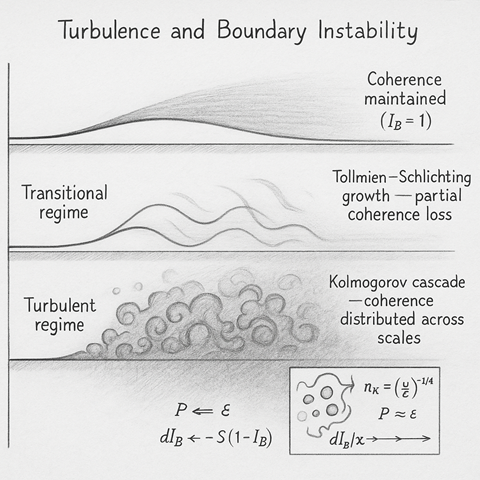
Turbulence is not chaos — it is coherence in transition.
Where laminar flow holds memory in smooth curvature, turbulence fragments it into smaller coherent packets.
Each eddy, wave, and fluctuation represents a partial memory of the original flow, carried across scales until dissipation finally erases it as heat.
In this view, turbulence is the recursive breakdown of boundary coherence — energy remembered imperfectly in ever smaller geometric echoes.
When a flow is laminar, the boundary is calm, and every layer moves predictably over the next.
Viscosity sustains perfect information exchange between layers — each velocity profile acts as a stable curvature field.
The momentum flux is coherent and continuous:
$$ \tau = \mu\,\frac{dU}{dy}, \qquad p + \frac{1}{2}\rho U^2 = \text{constant}. $$
As long as the Reynolds number stays low () for external surfaces, for boundary layers), perturbations decay rather than amplify.
The boundary holds its structural memory — coherence dominates inertia.
At higher Reynolds numbers, small disturbances begin to amplify.
Two primary families of instability appear:
Each wave represents a local coherence defect: a place where the boundary’s memory cannot maintain alignment across the flow.
When these defects multiply, laminar structure fragments — intermittency grows — and turbulence emerges.
Intermittency rises from 0 to 1 as:
$$ \chi = f(\mathrm{Re}_\theta, \beta_{\mathrm{APG}}, \text{inflection}). $$
marking the smooth transition from coherent to chaotic boundary geometry.
At equilibrium:
$$ P \approx \varepsilon. $$
The turbulence maintains a constant energy flux through scales — a cascade of coherence.
Large eddies inherit structure from mean flow; small eddies inherit from larger ones, each layer storing partial memory of motion.
Kolmogorov’s smallest scale defines the limit of coherence:
$$ \eta_K = \left(\frac{\nu^3}{\varepsilon}\right)^{1/4}. $$
At this size, viscosity erases structure completely — coherence becomes heat.
To quantify how turbulence destroys and rebuilds structure, we use the boundary coherence index .
The decay of is driven by both shear and adverse pressure gradient (APG):
$$ \frac{dI_B}{dx} = -\big(0.4\,S + 0.6\,\beta_{\mathrm{APG}}\big)\,(1 - I_B). $$
where is a non-dimensional shear rate and measures the severity of pressure recovery.
As falls below 0.6, the boundary can no longer sustain attachment — flow separates and eddies fill the wake.
Turbulence can be seen as a hierarchy of coherent memories:
Large eddies → smaller eddies → dissipative micro-vortices.
Each level translates curvature into finer structure, preserving the total energy flux but dividing the information.
This recursive geometry mirrors the holographic encoding of motion:
every substructure contains a reduced but consistent representation of the whole.
At the macroscopic level, this appears as random motion;
at the coherence level, it is a self-similar cascade of structure — order, distributed across scale.
As the flow encounters an adverse pressure gradient (APG), the outer flow decelerates while the near-wall flow remains slow.
Momentum transfer fails, and the flow reverses direction.
This creates a pocket of negative shear, an inflection point, and finally vortex shedding.
The Clauser parameter quantifies the onset:
$$ \beta_{\mathrm{APG}} = \frac{\theta}{\tau_w}\, \frac{dp}{dx}. $$
When and , separation begins — coherence has fully detached from the surface.