
Chapter 3
Alpha/Beta Spectra and Energy Quantisation

Complex and Cosmological Systems
Author: Mark Anthony Higgins
© Mark Anthony Higgins 11 October 2025
Revised Date: 23 February 2026
Audio Overview
Flow Algebra
flow "AlphaBeta_Spectra_EnergyQuantisation"

# ---------- STATES ----------
state:
  # nuclide / energetics
  nucleus.Z: int
  nucleus.N: int
  Q.value: float                     # decay Q for active branch (MeV)
  level.set: set[level]              # {E_ex, Jπ, branch}
  branch.table: map[channel, float]  # branching ratios (sum ≤ 1)
  channel.active: str?               # "alpha" | "beta_minus" | "beta_plus" | "EC" | "gamma"

  # sampled event kinematics (per tick if simulating)
  Ee: float                          # electron/positron kinetic energy
  Enu: float                         # neutrino energy (β channels)
  Eα: float                          # alpha kinetic energy
  Eγ: float                          # gamma energy
  Erecoil: float                     # nuclear recoil
  Elevel: float                      # selected excited level energy

  # spectral accumulators (ideal pre-detector)
  spec.alpha_lines: list[(E:float, weight:float)]
  spec.beta_e_hist: histogram        # electron/positron energy spectrum
  spec.gamma_lines: list[(E:float, weight:float)]
  spec.XR_Auger_lines: list[(E:float, weight:float)]  # from EC

  # detector model
  det.model: "gaussian" | "voigt"
  det.FWHM_keV: float                # resolution at reference energy
  det.ref_E_keV: float               # energy where FWHM_keV applies
  det.resolution_law: "sqrt" | "linear" | "constant"
  det.eta_tail: float                # low-energy tail fraction (0..1), optional

  # quantisation / calibration
  bin.Emin_keV: float
  bin.Emax_keV: float
  bin.N: int
  bin.edges: array[float]
  bin.centres: array[float]
  calib.gain: float                  # keV/channel
  calib.offset: float                # keV
  calib.nonlinearity: float          # small quadratic term (keV^-1), optional

  # physics modifiers
  Fermi.Zeff: float                  # effective Z for F(Z,E)
  shape_factor.kind: "allowed" | "first_forbidden" | "custom"
  shape_factor.C: fn(E)->float       # multiplicative spectral shape
  screening.S: fn(E)->float          # atomic screening correction
  radiative.R: fn(E)->float          # radiative (inner brems) correction
  endpoint.correction: fn()->float   # tiny shifts (recoil, screening) at endpoint

  # normalisation / runtime
  activity.Bq: float                 # events per second (for cps)
  live_time.s: float
  dead_time.frac: float              # 0..1
  pileup.rate: float                 # events/s (optional)

  # outputs (post-detector, quantised)
  spectrum.alpha_counts: array[float]  # binned counts
  spectrum.beta_counts: array[float]
  spectrum.gamma_counts: array[float]
  spectrum.total_counts: array[float]

# ---------- PARAMETERS ----------
params:
  me_keV: 510.99895                  # electron rest mass
  alpha_mass_keV: 3727.379           # alpha rest mass
  c2: 1.0                            # MeV units (natural)
  N_MC: int                          # Monte Carlo samples for spectra build
  voigt.eta: float                   # Lorentzian fraction if det.model="voigt"

# ---------- INVARIANTS ----------
invariant:
  - sum(branch.table.values) ≤ 1 + 1e-9
  - for α:  Q.value = Eα + Erecoil + Elevel    # (per event)
  - for β−: Q.value = Ee + Enu + Erecoil + Elevel
  - for β+: Q.value = Ee + Enu + 2*params.me_keV/1000 + Erecoil + Elevel
  - Ee ≥ 0, Eα ≥ 0, Eγ ≥ 0, Erecoil ≥ 0, Elevel ≥ 0
  - β endpoints: E0 = Q.value - Elevel - endpoint.correction() ≥ 0
  - histogram area ∝ expected decays after live time and dead-time losses

# ---------- TRANSFORMS ----------
transform:

  initialise_bins:
    do:
      bin.edges   = linspace(bin.Emin_keV, bin.Emax_keV, bin.N+1)
      bin.centres = 0.5*(bin.edges[:-1] + bin.edges[1:])

  choose_channel:
    do:
      channel.active = random_weighted_pick(branch.table)
      if channel.active == null: channel.active = "gamma"  # if pure isomeric γ

  pick_level:
    do:
      # sample nuclear level from level.set, weighted by branch × level.branch
      L = random_weighted_pick({lvl: lvl.branch for lvl in level.set})
      Elevel = L.E_ex

  alpha_event:
    pre:
      require channel.active == "alpha"
    do:
      # two-body kinematics → sharp line, split with recoil
      Eα = Q.value - Elevel - Erecoil_alpha(Q.value, nucleus.Z, nucleus.N)
      append(spec.alpha_lines, (E=to_keV(Eα), weight=1.0))

  beta_event:
    pre:
      require channel.active in ["beta_minus","beta_plus"]
    do:
      E0 = Q.value - Elevel - endpoint.correction()
      require E0 > 0
      # sample Ee from allowed/forbidden spectrum
      # S(E) ∝ F(Z,E) * p * (E+me)^k * (E0 - E)^2 * shape_factor.C(E) * screening.S(E) * radiative.R(E)
      Ee = sample_beta_energy(E0, Fermi.Zeff, shape_factor, screening, radiative, kind=channel.active)
      add_to_hist(spec.beta_e_hist, to_keV(Ee), weight=1.0)

  EC_event:   # electron capture → characteristic X-ray/Auger lines
    pre:
      require channel.active == "EC"
    do:
      lines = atomic_relaxation_lines(nucleus.Z)  # Kα, Kβ, L..., Auger
      for (E, w) in lines:
        append(spec.XR_Auger_lines, (E=E, weight=w))

  gamma_event:
    pre:
      require channel.active == "gamma"
    do:
      Eγ = Elevel   # de-excitation
      append(spec.gamma_lines, (E=to_keV(Eγ), weight=1.0))

  build_spectra_MC:
    do:
      for i in range(params.N_MC):
        choose_channel()
        pick_level()
        match channel.active:
          - "alpha":        alpha_event()
          - "beta_minus":   beta_event()
          - "beta_plus":    beta_event()
          - "EC":           EC_event()
          - "gamma":        gamma_event()

  apply_detector_response:
    do:
      # 1) start with zeros
      spectrum.alpha_counts = zeros(bin.N)
      spectrum.beta_counts  = zeros(bin.N)
      spectrum.gamma_counts = zeros(bin.N)

      # 2) convolve ideal lines/spectra with detector kernel (energy-dependent σ)
      for (E, w) in spec.alpha_lines:
        K = detector_kernel(E, bin.centres, det.FWHM_keV, det.ref_E_keV, det.resolution_law, det.model, params.voigt.eta, det.eta_tail)
        spectrum.alpha_counts += w * K

      # β: take histogram then smooth by kernel per bin centre
      spectrum.beta_counts += convolve_hist(spec.beta_e_hist, bin.centres, det.FWHM_keV, det.ref_E_keV, det.resolution_law, det.model, params.voigt.eta, det.eta_tail)

      # γ & EC lines
      for (E, w) in spec.gamma_lines:
        K = detector_kernel(E, bin.centres, det.FWHM_keV, det.ref_E_keV, det.resolution_law, det.model, params.voigt.eta, det.eta_tail)
        spectrum.gamma_counts += w * K
      for (E, w) in spec.XR_Auger_lines:
        K = detector_kernel(E, bin.centres, det.FWHM_keV, det.ref_E_keV, det.resolution_law, det.model, params.voigt.eta, det.eta_tail)
        spectrum.gamma_counts += w * K   # included in same panel by default

  calibrate_and_quantise:
    do:
      # Map true keV → channel space, then back via gain/offset/nonlinearity to mimic ADC quantisation
      # Here we assume bins are already in keV; nonlinearity can warp counts slightly across bins if desired.
      if calib.nonlinearity != 0:
        warp_bins(bin.centres, calib.nonlinearity)

  scale_counts_to_cps:
    do:
      scale = activity.Bq * live_time.s * (1 - dead_time.frac) / params.N_MC
      spectrum.alpha_counts *= scale
      spectrum.beta_counts  *= scale
      spectrum.gamma_counts *= scale
      spectrum.total_counts  = spectrum.alpha_counts + spectrum.beta_counts + spectrum.gamma_counts

# ---------- MONITORS ----------
monitor:
  alpha_line_index:
    observe: [spec.alpha_lines]
    report: "Expected α line positions (keV) and relative weights before detector broadening."

  beta_endpoint_check:
    observe: [Q.value, Elevel]
    report: "Computed β endpoint E0 per level; ensure histograms cut off at E0 (post-kernel may bleed slightly)."

  resolution_health:
    observe: [det.FWHM_keV, det.resolution_law]
    report: "Check σ(E) scaling; too broad smears discrete lines, too narrow hides realism."

  normalisation:
    observe: [activity.Bq, live_time.s, dead_time.frac]
    report: "Counts should scale linearly with activity×live_time×(1-dead_time)."

# ---------- NOTES ----------
note:
  - α spectra are **discrete**: two-body kinematics → sharp lines; detector turns them into Gaussians/Voigts.
  - β spectra are **continuous** up to endpoint E0; shape ∝ Fermi function × phase space × (forbiddenness) × small corrections.
  - EC yields **characteristic X-ray/Auger** lines; include in γ panel or separate.
  - Recoil and excited-level energy subtract from particle kinetic energy, shifting α lines and β endpoints.
  - Detector resolution often follows σ(E) ∝ √E; choose det.resolution_law="sqrt" for scintillators/semiconductors.
  - Apply small endpoint corrections (screening, radiative, recoil) if comparing to high-precision data.
  - For β+ include the 2me term in Q accounting; if modelling annihilation, add 511 keV γ lines (2× or 3× topology).
What this flow captures (intent)

AlphaBeta_Spectra_EnergyQuantisation describes how radioactive decays translate into measurable energy spectra, bridging internal coherence loss with external quantised emissions.

It separates the discrete, two-body α spectra from the continuous, many-body β spectra, adding the detector’s energy resolution and quantisation steps.
This connects nuclear boundary transitions to the actual lines and shapes seen in laboratory spectrometers.


Core intuition (HST view)
  • Each decay event is a coherence redistribution: the nucleus resolves internal curvature stress by emitting a quantised packet of energy.
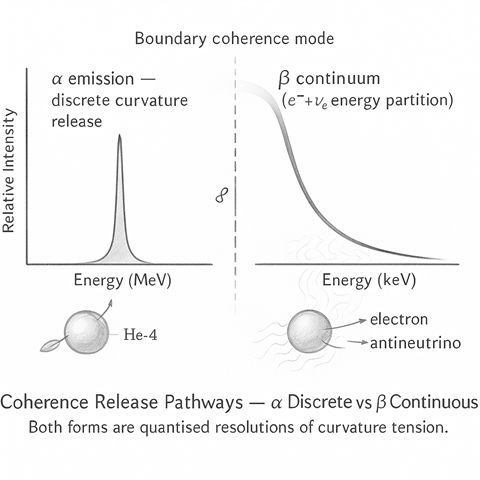
  • α decay produces sharply defined lines because the emission involves two coherent bodies only — the daughter nucleus and the α cluster — meaning all curvature release is discretely channelled.
  • β decay involves internal topology flips (n↔p) coupled to a continuous lepton field; energy is spread probabilistically between the electron (or positron) and neutrino, giving a smooth spectral curve.
  • γ emission and electron capture (EC) appear as secondary quantised lines, completing the curvature relaxation sequence.
  • Detector response and quantisation mimic how coherent field packets become discrete digital observables, linking physical emission to human measurement.
Spectral structure explained
  • α lines:
    Each line corresponds to a fixed Q-value minus recoil and level energy.
    Multiple lines arise from decays feeding excited states in the daughter nucleus.
    In the flow, these appear as delta functions broadened by the detector kernel.
  • β spectra:
    Derived from phase-space and Fermi statistics. The shape is
    S(E) ∝ F(Z,E) · p(E+me)²(E0−E)² · C(E) with corrections (screening, radiative).
    In HST terms, this continuous spread reflects distributed boundary dephasing—the coherence release is partial and probabilistic rather than singular.
  • γ and EC lines:
    Represent curvature relaxation of specific levels; electron capture leads to characteristic X-ray and Auger cascades.
    These transitions show that coherence can collapse inward (via capture) as well as outward (via emission).

Energy quantisation & measurement

Energy is not continuous in emission space — it is quantised by boundary geometry.
Each allowed emission corresponds to an integer multiple of the minimal curvature packet consistent with conservation and topology.
However, when coupled to lepton fields or detectors, this quantisation appears continuous because the measurement integrates over a range of micro-states.

The flow’s calibrate_and_quantisesection emulates this: energy packets are mapped through a gain, offset, and mild non-linearity to create digitised ADC channels — a mirror of how the physical continuum becomes discrete data.


Parameter guidance
Symbol / FieldMeaningTypical Impact

Fermi.Zeff

effective charge for Coulomb corrections
shifts β spectrum slope

shape_factor.kind

allowed / forbidden
modifies high-energy tail

det.FWHM_keV

detector resolution
broadens lines, smears endpoints

calib.gain, offset

energy-to-channel map
sets calibration curve

activity.Bq × live_time.s

scales total counts
sets overall normalisation

Keep the resolution model realistic (sqrt for semiconductor, linear for scintillator).
If det.eta_tail > 0, the flow reproduces the faint low-energy tails common in real detectors.


Monitors and diagnostics
  • alpha_line_index — confirms correct Q-derived α energies before convolution.
  • beta_endpoint_check — verifies energy conservation and visible endpoint cutoff.
  • resolution_health — ensures detector kernel broadening is physically reasonable.
  • normalisation — checks event scaling with activity and live time.

When plotted, the total spectrum should show:

  • sharp α peaks at discrete energies,
  • smooth β continua tapering to Q-value endpoints,
  • γ and X-ray lines superimposed at characteristic energies

Conceptual link to coherence physics

In the HST framework, each spectral line or continuum section is a record of coherence relaxation.
α lines mark complete boundary restorations;
β spectra trace distributed phase equalisation through weak topologies;
γ lines mark fine curvature smoothing;
and the quantised detector readout represents the final collapse of field coherence into information.

Thus, the same process that drives nuclear decay also defines the quantum of measurable knowledge — energy quantisation is the signature of coherence resolving into countable form.


Worked Example — Po-210 (α) vs Sr-90/Y-90 (β⁻)
Case 1 — Po-210 (α decay)

Physical context:

Polonium-210 decays almost exclusively by α emission to lead-206 with a half-life of 138 days and a Q-value of 5.407 MeV.
From the HST view, the nucleus reaches a global-curvature tipping point and releases a perfectly coherent four-nucleon packet (the α cluster), restoring boundary symmetry.

Initialisation (simplified)

nucleus.Z = 84; nucleus.N = 126
Q.value = 5.407
level.set = [{E_ex:0.0, Jπ:"0+", branch:1.0}]
branch.table = {"alpha":1.0}
det.model = "gaussian"; det.FWHM_keV = 60; det.resolution_law="sqrt"
bin.Emin_keV=5000; bin.Emax_keV=5600; bin.N=300
activity.Bq = 1.0e6; live_time.s = 10.0; dead_time.frac = 0.02
params.N_MC = 100000
Expected behaviour:
  • A single dominant α line appears near 5304 keV after recoil and detector broadening.
  • The boundary integrity in the source nucleus falls, expels the α cluster, and rebounds—one clean curvature discharge.
  • The spectrum is essentially Gaussian:
    narrow, bright, and self-limiting—evidence of a quantised two-body release.
Interpretation:

Every α event is the same coherence event repeated—energy quantisation made visible.
Detector resolution simply blurs the precision of the field packet’s transition.


Case 2 — Sr-90 → Y-90 → Zr-90 (β⁻ chain)

Physical context:

Strontium-90 decays to Yttrium-90 (Q = 0.546 MeV, t₁/₂ = 28.8 y), then Yttrium-90 decays to Zirconium-90 (Q = 2.28 MeV, t₁/₂ = 64 h).

Each stage emits β⁻ particles with continuous spectra up to their respective endpoints.

Initialisation (simplified)

nucleus.Z = 38; nucleus.N = 52
Q.value = 0.546
branch.table = {"beta_minus":1.0}
Fermi.Zeff = 39.0
shape_factor.kind = "allowed"
det.model="gaussian"; det.FWHM_keV=50; det.resolution_law="sqrt"
bin.Emin_keV=0; bin.Emax_keV=600; bin.N=300
activity.Bq=5.0e5; live_time.s=10.0
params.N_MC=200000

Expected behaviour:

  • The β⁻ spectrum forms a smooth continuum from 0 → E₀ ≈ 546 keV, shaped by the Fermi function and phase space.
  • Adding Y-90’s branch (Q = 2.28 MeV) overlays a broader, higher-energy continuum.
  • The spectrum’s soft tail reflects distributed phase dispersion—each decay releases a fraction of the internal curvature, not a single packet.
  • Slight curvature near endpoint E₀ shows screening and recoil corrections.

Interpretation:

β spectra embody probabilistic coherence resolution: instead of ejecting one defined cluster, the nucleus balances its boundary by sharing energy across coupled fields (electron + neutrino).   The resulting continuum demonstrates that even within randomness, the total coherence release remains quantised—its sum across events equals the same Q partition law that governs α lines.


Comparison and insight
Featureα Decay (Po-210)β Decay (Sr-90/Y-90)
Emission topology
Two-body
Three-body
Spectral form
Discrete line(s)
Continuous continuum
Coherence mode
Singular release
Distributed release
Dominant coupling
Strong (boundary)
Weak (topological)
Measurement signature
Sharp peak
Smooth cutoff
HST interpretation
Boundary collapse
Internal topology re-balancing

Closing reflection

Both spectra are expressions of the same law of coherence:
when boundary integrity fails, energy leaves in quantised packets whose statistical distributions are set by the geometry of release.

α lines show coherence resolving in one breath; β continua show it as a harmonic decay through phase dispersion.
The apparent contrast between discrete and continuous spectra is not a contradiction—it is the same coherence physics viewed through different coupling densities.

Kireth Research
38 Thorndale Croft, Wetwang, Driffield
East Riding of Yorkshire YO25 9XZ
Designed By