Chapter 56
Schrödinger Flow Equation
Quantum Coherence and Boundary Systems
Author: Mark Anthony Higgins
© Mark Anthony Higgins 11 October 2025
Revised Date: 23 February 2026
flow "Schrödinger Flow Equation" v1.0
# ---------- PURPOSE ----------
# Models the Schrödinger equation as a coherence-preserving flow in complex phase space.
# The equation governs time evolution of a wavefunction ψ under a potential V(x,t):
# iħ ∂ψ/∂t = [ - (ħ² / 2m) ∇² + V(x,t) ] ψ
# In the coherence framework, this expresses local conservation of phase curvature — the continuous evolution of boundary memory.
# IB tracks coherence integrity of the wavefunction (1 = perfectly coherent, <1 = partial decoherence or environmental coupling).
# ---------- PARAMETERS ----------
params:
units: "SI"
ħ: real = 1.054_571_817e-34 # reduced Planck constant [J·s]
m: positive # particle mass [kg]
V: func?(x:real,t:real)->real # potential energy function [J]
IB: 0.0..1.0 = 1.0 # wavefunction coherence index
λ_decoh: nonnegative = 0.0 # decoherence rate [s^-1]
dt: positive? # timestep [s]
include_probability_flow: bool = true
# ---------- STATE ----------
state Quantum:
ψ: complex # wavefunction ψ(x,t)
ρ: real # probability density |ψ|²
J: real # probability current density [A/m²]
Hψ: complex # Hamiltonian operator applied to ψ
phase: real # instantaneous phase arg(ψ)
IB_rate: real # rate of coherence change
norm: real # normalisation ∫|ψ|² dx
energy_expectation: real # ⟨E⟩ = ⟨ψ|H|ψ⟩
regime: str # "stationary", "dynamic", or "decohering"
# ---------- INVARIANTS ----------
invariants:
# Schrödinger time evolution (differential form)
Quantum.Hψ = -(params.ħ**2 / (2 * params.m)) * ∇²(Quantum.ψ) + params.V(x,t) * Quantum.ψ
iħ ∂ψ/∂t = Quantum.Hψ
Quantum.ψ(t+dt) = Quantum.ψ(t) + (-i/params.ħ) * Quantum.Hψ * (params.dt or 1)
# Probability density and current (continuity equation)
Quantum.ρ = |Quantum.ψ|^2
if params.include_probability_flow:
Quantum.J = (params.ħ / params.m) * Im(conjugate(Quantum.ψ) * ∇Quantum.ψ)
# Continuity relation (local conservation)
∂Quantum.ρ/∂t + ∇⋅Quantum.J = 0
# Normalisation check
Quantum.norm = ∫Quantum.ρ dx
# Expected energy
Quantum.energy_expectation = Re(∫conjugate(Quantum.ψ) * Quantum.Hψ dx)
# Coherence decay (optional)
if params.λ_decoh > 0 and params.dt is defined:
params.IB = clamp(params.IB - params.λ_decoh * (1 - params.IB) * params.dt, 0, 1)
Quantum.IB_rate = -params.λ_decoh * (1 - params.IB)
# Regime classification
if params.IB == 1:
Quantum.regime = "stationary"
elif params.IB > 0.5:
Quantum.regime = "dynamic"
else:
Quantum.regime = "decohering"
# ---------- TRANSFORMS ----------
transforms:
evolve_time_step:
comment: "Advance ψ(x,t) one timestep via unitary evolution operator."
Quantum.ψ = exp(-i * H * (params.dt or 1) / params.ħ) * Quantum.ψ
apply_potential:
comment: "Update ψ(x,t) under a new potential landscape."
Quantum.Hψ = -(params.ħ**2 / (2 * params.m)) * ∇²(Quantum.ψ) + params.V(x,t) * Quantum.ψ
normalise_wavefunction:
comment: "Renormalise ψ to ensure total probability = 1."
Quantum.ψ = Quantum.ψ / sqrt(∫|Quantum.ψ|² dx)
Quantum.norm = 1
decay_coherence:
comment: "Apply environmental decoherence to wavefunction coherence index."
params.IB = clamp(params.IB - 0.01 * (1 - params.IB), 0, 1)
# ---------- MONITORS ----------
monitors:
probability_conservation:
assert abs(d/dt(Quantum.norm)) <= 1e-9
comment: "Total probability conserved under unitary evolution."
energy_consistency:
assert Quantum.energy_expectation >= 0
coherence_bounds:
assert 0 <= params.IB <= 1
phase_tracking:
comment: "Track continuous phase evolution of ψ across time."
# ---------- SCENES ----------
scenes:
free_particle:
given params:
m: 9.11e-31
V: (x,t)->0
IB: 1.0
expect:
Quantum.regime = "stationary"
comment: "Free evolution of plane wave — uniform phase velocity."
harmonic_oscillator_ground_state:
given params:
m: 9.11e-31
V: (x,t)->0.5 * m * (ω₀^2) * x^2
IB: 1.0
expect:
Quantum.energy_expectation = 0.5 * ħ * ω₀
comment: "Stationary Gaussian wavefunction — minimal phase curvature."
wavepacket_dispersion:
given params:
m: 9.11e-31
V: (x,t)->0
IB: 1.0
expect:
Quantum.regime = "dynamic"
comment: "Wavepacket spreads over time — curvature unfolds coherently."
decohering_wavefunction:
given params:
m: 9.11e-31
V: (x,t)->0
IB: 0.7
λ_decoh: 0.05
dt: 1.0
enable:
- decay_coherence
expect:
Quantum.regime = "decohering"
comment: "Environmental coupling diffuses phase — probability conserved but coherence fades."
# ---------- NOTES ----------
notes:
- **Schrödinger Equation:**
\[
i\hbar\frac{\partial\psi}{\partial t}
= \left[-\frac{\hbar^2}{2m}\nabla^2 + V(x,t)\right]\psi
\]
Describes the continuous evolution of the wavefunction ψ in time.
- **Probability Continuity:**
\[
\frac{\partial\rho}{\partial t} + \nabla\cdot\mathbf{J} = 0, \quad
\rho = |\psi|^2, \quad
\mathbf{J} = \frac{\hbar}{m}\Im(\psi^*\nabla\psi)
\]
Ensures conservation of total probability across all space.
- **Energy Expectation:**
\[
\langle E \rangle = \int \psi^*(x) H \psi(x)\,dx
\]
- **Coherence Law:**
\[
\dot{I_B} = -\lambda (1 - I_B)
\]
Models gradual decoherence from environmental interaction.
- **Interpretation (HST–Flow):**
The Schrödinger equation is not just a temporal rule — it is **phase continuity in curvature form**.
The wavefunction ψ describes a field of recursive curvature coherence, with time evolution preserving the total boundary memory (probability).
When \(I_B = 1\), the flow is unitary — a perfect coherence loop.
When \(I_B < 1\), the loop opens — phase information leaks outward, and interference visibility decays.
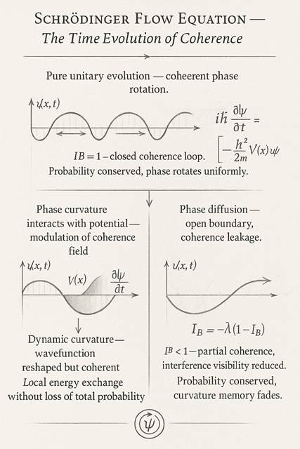
- **Visualization:**
- Left: ψ(x,t) as a complex plane wavefront (pure state).
- Middle: ψ evolving under potential (curvature modulation).
- Right: ψ amplitude fading with phase blur as IB decreases (decoherence).
The Schrödinger equation is not just the engine of quantum mechanics — it is the grammar of coherence through time.
It describes how phase information flows continuously across a boundary without loss, defining the dynamic equilibrium between curvature, potential, and probability.
In the HST view, it expresses recursive phase continuity — the way reality remembers its own curvature through the wavefunction.
The time-dependent Schrödinger equation governs how a system’s state evolves:
\[ i\hbar \frac{\partial \psi}{\partial t} = \left[ -\frac{\hbar^2}{2m}\nabla^2 + V(x,t) \right] \psi \]
It ensures that the probability density remains constant across time, preserving total normalisation.
This is captured by the continuity equation:
\[ \frac{\partial \rho}{\partial t} + \nabla \cdot \mathbf{J} = 0, \qquad \mathbf{J} = \frac{\hbar}{m} \Im(\psi^* \nabla \psi) \]
where is the probability current — the flux of coherence through configuration space.
Every solution to the Schrödinger equation represents a stable coherence flow — a pattern of phase curvature sustained by balance between potential energy and wave dispersion.
In the HST–Flow framework, the wavefunction ψ is not a mathematical abstraction but a field of curvature memory.
Its amplitude represents spatial distribution of coherence, and its phase represents the local curvature orientation of that coherence in time.
The term describes how curvature diffuses spatially, while defines how the environment folds that curvature locally.
The imaginary unit i introduces rotation in the phase plane — a continual reorientation of curvature memory through time.
Thus, Schrödinger evolution is the rotation of coherence in complex space, where amplitude and phase exchange dynamically without loss.
The continuity equation is not merely statistical; it expresses the conservation of total curvature memory.
The “probability current” is a flux of coherence, transporting information across the field while maintaining global balance.
When the boundary is closed (no external interaction), this flow is perfectly unitary — coherence recirculates within the system, and .
When the system couples to an environment, boundary information leaks outward, lowering .
This is decoherence — open-boundary curvature diffusion rather than collapse.
A stationary state satisfies:
\[ H\psi = E\psi \]
and evolves only through global phase rotation:
\[ \psi(x,t) = \psi(x,0)e^{-iEt/\hbar} \]
Its curvature field is static — the internal boundary is in perfect self-equilibrium.
By contrast, a non-stationary wavepacket evolves dynamically.
Its curvature unfolds in time, redistributing coherence while still obeying the conservation of total probability.
This dynamic interplay between dispersion and potential defines temporal curvature modulation — the way reality maintains stability while constantly transforming itself.
No real system is perfectly isolated.
When environmental interaction introduces phase noise or entanglement with unobserved degrees of freedom, coherence gradually decays
\[ \dot{I_B} = -\lambda (1 - I_B) \]
The wavefunction no longer evolves purely unitarily — its internal curvature begins to blur.
Amplitude remains conserved (probability continuity still holds), but the sharpness of phase relation between points decreases.
The once-precise interference pattern becomes diffused, marking a transition from deterministic evolution to mixed behaviour.
In HST terms, this is the boundary opening its loop — curvature spreading into adjacent domains.
Decoherence is not destruction, only redistribution.
At its deepest level, the Schrödinger equation defines the flow of coherence between boundaries of curvature:
Together they form a balanced recursive loop: energy, curvature, and phase continually transform while preserving global integrity.
In HST language, this loop is the phase-space heartbeat of reality — the smallest dynamical process that can remember itself.
The Schrödinger equation is a law of phase continuity, not probability mysticism.
It ensures that curvature memory (ψ) evolves coherently through time, preserving the total boundary condition of existence.
In the HST–Flow interpretation:
Thus, the Schrödinger equation describes the time flow of coherence —
a self-consistent recursion where the universe continually rewrites itself without ever breaking its own symmetry.
The wavefunction does not predict the future — it preserves the memory of curvature as time unfolds.