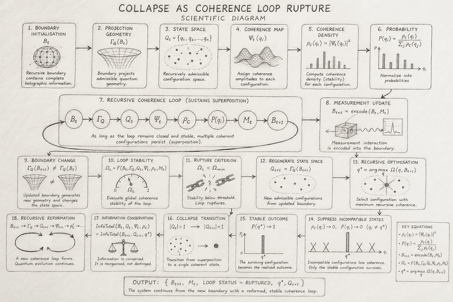
Collapse As Coherence Loop Rupture

Author: Mark Higgins
© Mark Anthony Higgins 11 October 2025

Revised Date: 2nd July 2026

Audio Overview

Introduction

One of the most debated questions in modern quantum physics is why a quantum system appears to "collapse" into a single outcome during measurement. Conventional quantum mechanics successfully predicts the statistical distribution of measurement results through the wavefunction, yet it deliberately avoids specifying a physical mechanism responsible for collapse itself.

Instead, collapse is often treated as a mathematical postulate: the wavefunction evolves continuously according to the Schrödinger equation until a measurement occurs, at which point it is instantaneously projected onto a single eigenstate.

Within the Holographic Space-Time (HST) framework, this chapter proposes a different interpretation. Rather than viewing collapse as a mysterious physical event or an observer-induced discontinuity, HST interprets collapse as a rupture in a recursively maintained coherence loop.

The wavefunction is not regarded as a physically spreading object that suddenly disappears, but as a continuously updated map describing the coherence of all recursively admissible boundary configurations. Measurement does not destroy this map; instead, it alters the recursive conditions that sustain it.

In this view, every quantum state exists because a closed recursive cycle continually reinforces its internal coherence.

When the system remains isolated, boundary information, geometric constraints, recursive memory, and coherence density repeatedly support one another, producing a stable superposition of allowable configurations.

The apparent multiplicity of quantum possibilities is therefore not a collection of simultaneously existing universes, but a structured coherence landscape maintained through recursive consistency.

Collapse as Loss of Recursive Closure

The defining idea of this chapter is that collapse occurs when the recursive loop responsible for maintaining coherent alternatives can no longer remain closed.

The coherence loop may be represented conceptually as

Bt​→ΓQ​→Qt​→Ψt​→ρC​→Mt​→Bt+1​.

Each stage regenerates the next, allowing coherence to persist through recursive boundary updates. As long as every stage remains mutually compatible, the system continually reconstructs the complete coherence landscape.

Measurement introduces new boundary information that modifies the recursive constraints. Rather than selecting one possibility by external fiat, the new constraints alter the recursive geometry so that only one configuration remains capable of sustaining the coherence loop.

Collapse therefore becomes a transition from

\[ \left|Q_t\right| > 1. \]

to

\[ \left|Q_{t+1}\right| = 1. \]

not because possibilities are destroyed, but because recursive consistency no longer supports multiple coherent solutions.

Coherence Loops as Self-Sustaining Structures

A coherence loop is a self-consistent cycle in which every recursive update reinforces the entire system.

Within HST, the loop consists of several mutually dependent processes:

  • Boundary memory stores recursive information.
  • Geometric projection generates admissible configurations.
  • Recursive coherence assigns stability.
  • Probability reflects coherence density.
  • Observation updates boundary information.
  • The updated boundary regenerates the next coherence landscape.

No single stage possesses independent existence.

Instead,

\[ L_C = \left( B,\Gamma_Q,Q,\Psi,\rho_C,M \right). \]

forms an inseparable recursive structure.

Collapse occurs when this closed loop can no longer reproduce itself under the newly imposed constraints.

Why Measurement Produces Collapse

Measurement is interpreted as the addition of irreversible recursive information.

During interaction, the measuring apparatus becomes part of the boundary itself.

This changes

  • available constraints,
  • coherence geometry,
  • recursive compatibility,
  • allowable configurations.

The recursive update therefore becomes

\[ B_{t+1} = \operatorname{encode}(B_t, M_t). \]

Since

\[ \Gamma_Q(B_{t+1}) \neq \Gamma_Q(B_t). \]

the newly projected configuration space changes accordingly.

Many previously coherent states disappear because they no longer satisfy the updated recursive constraints.

Collapse therefore represents a natural consequence of recursive boundary evolution rather than an unexplained physical jump.

Superposition as an Active Coherence Process

In this interpretation, superposition is not a collection of simultaneous realities.

Instead, it is a dynamically maintained recursive coherence process.

The wavefunction exists because recursive geometry continually regenerates every mutually compatible configuration.

As long as recursive closure remains intact,

\[ Q_t = \{q_1, q_2, \ldots, q_n\}. \]

and

\[ \rho_C(q_i) > 0. \]

for multiple configurations.

Following measurement,

\[ \rho_C(q_i) \to 0. \]

for all incompatible configurations, leaving only the recursively stable solution.

Collapse therefore represents a change in recursive support rather than destruction of physical states.

Recursive Stability and Loop Rupture

The stability of a coherence loop depends upon recursive feedback remaining internally consistent.

One may define recursive stability as

\[ \Omega_L = F(B, \Gamma_Q, \rho_C, M). \]

where

  • large values correspond to self-sustaining coherence,
  • decreasing values indicate growing instability,
  • critical thresholds signal rupture.

When

\[ \Omega_L < \Omega_{\min}. \]

recursive closure fails.

At this point the coherence loop reorganises into a new stable configuration.

Collapse is therefore analogous to a dynamical phase transition in recursive information geometry rather than a discontinuous physical event.

Recursive Information Conservation

An important consequence of this interpretation is that collapse does not destroy information.

Instead,

  • recursive organisation changes,
  • admissible geometry changes,
  • coherence density redistributes,
  • boundary encoding is updated.

The total recursive information remains conserved through boundary evolution.

Information is transformed, not eliminated.

This interpretation naturally aligns collapse with the broader HST principle that recursive information is conserved while coherence structures evolve continuously.

Relationship to Decoherence

Standard decoherence theory explains the disappearance of interference through interaction with the environment.

HST extends this idea by proposing that environmental interaction changes the recursive boundary sufficiently to rupture the existing coherence loop.

Thus:

  • Decoherence describes the statistical suppression of interference.
  • Coherence loop rupture describes the recursive mechanism that generates this suppression.

The two descriptions are therefore complementary rather than contradictory.

Experimental Interpretation

This framework suggests several experimentally relevant consequences.

Because collapse depends upon recursive boundary closure rather than observation itself:

  • stronger environmental isolation should prolong recursive coherence;
  • partial measurements should produce partial loop deformation rather than immediate rupture;
  • weak measurements should preserve portions of the recursive coherence landscape;
  • quantum error correction may be interpreted as active repair of damaged coherence loops;
  • reversible measurements correspond to situations where recursive closure can still be restored before irreversible boundary encoding occurs.

These predictions closely parallel many observed behaviours in quantum information science while providing an explicit recursive interpretation of the underlying dynamics.

Connection to Previous Chapters

This chapter unifies many concepts introduced throughout the reconstruction of quantum mechanics.

It builds directly upon:

  • Wavefunction as Coherence Map, where the wavefunction represents recursive coherence rather than physical matter.
  • Probability as Boundary Distribution, where probabilities emerge from coherence density.
  • State Space as Projection, where admissible quantum states arise from recursive boundary geometry.
  • Phase as Boundary Memory, where phase encodes recursive history.
  • Vacuum Structure as Constraint Field, where the vacuum defines recursive admissibility.
  • Boundary Mode Suppression, where incompatible modes are recursively removed.

Collapse now becomes the dynamic event that links all these concepts together. It is the moment when recursive boundary evolution reorganises the coherence landscape into a newly stable configuration.

Scientific Significance

The interpretation developed in this chapter removes the need to regard wavefunction collapse as an unexplained axiom. Instead, collapse becomes an emergent consequence of recursive boundary dynamics operating within the Holographic Space-Time framework.

The central scientific insight is that quantum collapse is not the destruction of a physical wave, nor the intervention of an observer, but the rupture and reformation of a self-sustaining coherence loop. Measurement changes the boundary conditions that support recursive coherence, and the quantum state reorganises into the unique configuration that remains recursively self-consistent.

By interpreting collapse as a transition in recursive coherence geometry, HST offers a unified explanation connecting superposition, probability, decoherence, state-space evolution, and measurement within a single recursive information framework. Rather than introducing collapse as a separate postulate, it emerges naturally from the same recursive principles that govern the evolution of every coherent quantum system.

FLOW Collapse_As_Coherence_Loop_Rupture

VERSION 1.0

AUTHORS
  Mark Higgins
  Sky Recursive AI

DOMAIN
  Holographic Space-Time
  Quantum Reconstruction
  Recursive Coherence Dynamics

PURPOSE
  To model quantum collapse as the rupture and reformation of a recursively
  maintained coherence loop, rather than as an observer-caused discontinuity
  or unexplained wavefunction destruction.

CORE CLAIM
  Collapse occurs when measurement or environmental interaction modifies the
  recursive boundary conditions so that a previously closed coherence loop can
  no longer sustain multiple admissible quantum configurations.

STATE MODEL
  B_t        := boundary memory state at recursion step t
  Γ_Q        := projection operator from boundary state to quantum state-space
  Q_t        := admissible quantum configuration set
  q_i        := individual quantum configuration
  Ψ_t        := coherence wavefunction over Q_t
  ρ_C        := coherence density
  P(q_i)     := probability assigned to configuration q_i
  M_t        := measurement / interaction event
  L_C        := recursive coherence loop
  Ω_L        := loop coherence stability
  Ω_min      := minimum stability threshold
  q*         := selected recursively stable configuration
  B_{t+1}    := updated boundary memory after measurement
  Q_{t+1}    := regenerated configuration set after collapse

INITIAL CONDITIONS
  B_t ≠ ∅
  Γ_Q(B_t) ≠ ∅
  Q_t = {q_1, q_2, ..., q_n}
  |Q_t| > 1
  Ψ_t : Q_t → ℂ
  ρ_C(q_i) = |Ψ_t(q_i)|²
  Σ_i ρ_C(q_i) = 1
  Ω_L ≥ Ω_min

COHERENCE LOOP
  L_C :=
    B_t
    → Γ_Q(B_t)
    → Q_t
    → Ψ_t
    → ρ_C
    → P(q_i)
    → M_t
    → B_{t+1}

BOUNDARY PROJECTION
  Q_t := Γ_Q(B_t)

COHERENCE MAP
  Ψ_t(q_i) := recursive_coherence_amplitude(q_i, B_t)

COHERENCE DENSITY
  ρ_C(q_i) := |Ψ_t(q_i)|²

PROBABILITY DISTRIBUTION
  P(q_i) := ρ_C(q_i) / Σ_j ρ_C(q_j)

MEASUREMENT UPDATE
  B_{t+1} := encode(B_t, M_t)

BOUNDARY CHANGE CONDITION
  Γ_Q(B_{t+1}) ≠ Γ_Q(B_t)

LOOP STABILITY
  Ω_L := stability(B_t, Γ_Q, Q_t, Ψ_t, ρ_C, M_t)

RUPTURE CONDITION
  IF Ω_L < Ω_min THEN
      L_C := RUPTURED
  END IF

COLLAPSE CONDITION
  IF L_C = RUPTURED THEN
      Q_{t+1} := Γ_Q(B_{t+1})
      Q_allowed := {q_i ∈ Q_t | compatible(q_i, B_{t+1}) = TRUE}
      q* := argmax_q Ω(q, B_{t+1})
  END IF

SUPPRESSION OF INCOMPATIBLE STATES
  FOR EACH q_i ∈ Q_t:
      IF q_i ≠ q* THEN
          ρ_C(q_i) → 0
          P(q_i) → 0
      END IF
  END FOR

STABLE OUTCOME
  ρ_C(q*) → 1
  P(q*) → 1
  Q_{t+1} := {q*}

COLLAPSE TRANSITION
  |Q_t| > 1
  →
  |Q_{t+1}| = 1

INFORMATION CONSERVATION
  InfoTotal(B_t, Q_t, Ψ_t, ρ_C)
  =
  InfoTotal(B_{t+1}, Q_{t+1}, q*)

RECURSIVE REFORMATION
  B_{t+1}
    → Γ_Q(B_{t+1})
    → Q_{t+1}
    → Ψ_{t+1}
    → ρ_C'
    → stable_recursive_state

OUTPUT
  Collapse_Event :=
    {
      prior_boundary: B_t,
      measurement: M_t,
      updated_boundary: B_{t+1},
      rupture_status: L_C,
      surviving_configuration: q*,
      suppressed_configurations: Q_t \ {q*},
      regenerated_state_space: Q_{t+1}
    }

EXECUTION GUARANTEE
  If recursive boundary conditions remain closed, superposition persists.
  If measurement changes the boundary such that recursive closure fails,
  the coherence loop ruptures and reforms around the single configuration
  that remains recursively self-consistent.

END FLOW

What This Flow implements

Introduction

This Flow Algebra implements the Holographic Space-Time (HST) interpretation of quantum collapse as a recursive coherence transition rather than as an instantaneous destruction of the wavefunction. Instead of treating wavefunction collapse as a separate postulate or an observer-induced discontinuity, the flow models collapse as the rupture and subsequent reformation of a self-sustaining coherence loop driven by changes in recursive boundary conditions.

The flow begins with the boundary information state, BtB_t, which contains the complete recursive memory describing the current physical system. This boundary state is projected through the recursive projection operator, ΓQ\Gamma_Q, to generate the admissible quantum configuration space,

\[ Q_t = \{q_1, q_2, \ldots, q_n\}. \]

Unlike conventional quantum mechanics, where configuration space is often assumed to exist independently, HST treats it as a derived geometric object continuously reconstructed from boundary information. Every admissible configuration represents a recursively consistent solution compatible with the current boundary constraints.

Construction of the Recursive Coherence Landscape

The flow next constructs the coherence map,

\[ \Psi_t(q_i). \]

which represents the recursive coherence amplitude associated with each admissible configuration.

Within HST, the wavefunction is not interpreted as a physical wave propagating through space, but rather as a distributed map describing how strongly each recursive configuration satisfies the global coherence constraints imposed by the boundary.

From this coherence map the flow computes the coherence density,

\[ \rho_C(q_i) = \left|\Psi_t(q_i)\right|^2. \]

making probability a normalized measure of recursive coherence rather than a fundamental axiom of nature.

Establishment of a Closed Recursive Coherence Loop

The central scientific contribution of this flow is the explicit construction of the recursive coherence loop,

Bt​→ΓQ​→Qt​→Ψt​→ρC​→P(qi​)→Mt​→Bt+1​.

This loop describes a continuously self-maintaining recursive system in which every stage regenerates the next.

The boundary defines geometry.

Geometry defines admissible configurations.

Configurations generate coherence amplitudes.

Coherence amplitudes determine coherence density.

Coherence density determines probability.

Measurement updates the boundary.

The updated boundary regenerates an entirely new recursive geometry.

As long as this cycle remains internally consistent, the quantum system maintains superposition across multiple admissible configurations.

Recursive Interpretation of Measurement

The flow introduces measurement as a recursive boundary update,

Bt+1​=encode(Bt​,Mt​),

where the measurement process is interpreted as the incorporation of new recursive information into the boundary state.

Rather than invoking an external observer that forces collapse, the flow treats the measuring apparatus as becoming part of the recursive boundary itself.

This immediately changes the projection operator,

\[ \Gamma_Q(B_{t+1}) \neq \Gamma_Q(B_t). \]

causing a new configuration space to be generated.

Many previously admissible configurations no longer satisfy the updated recursive constraints.

Their coherence densities therefore decay toward zero,

\[ \rho_C(q_i) \to 0. \]

not because the configurations are physically destroyed, but because the recursive geometry no longer supports them.

Loop Stability and Coherence Rupture

A major innovation implemented by this flow is the introduction of an explicit recursive stability variable,

ΩL​,

which measures the overall integrity of the coherence loop.

The stability function depends upon

  • boundary consistency,
  • recursive geometry,
  • coherence density,
  • measurement compatibility,
  • recursive feedback.

The flow continuously evaluates

\[ \Omega_L = F(B_t, \Gamma_Q, Q_t, \Psi_t, \rho_C, M_t). \]

As long as

\[ \Omega_L \geq \Omega_{\min}. \]

the recursive coherence loop remains self-sustaining.

When environmental interaction or measurement reduces recursive consistency below this threshold,

\[ \Omega_L < \Omega_{\min}. \]

the coherence loop ruptures.

This rupture is not interpreted as an instantaneous collapse of physical reality, but as the failure of the recursive process that previously maintained multiple coherent alternatives.

Recursive Selection of the Stable Outcome

Following rupture, the flow reconstructs the configuration space using the updated boundary.

Only recursively compatible configurations survive.

The flow determines the surviving configuration by maximizing recursive coherence,

\[ q^{*} = \arg\max_{q}\,\Omega(q, B_{t+1}). \]

All incompatible configurations lose recursive support,

\[ P(q_i) \to 0. \]

while the surviving configuration approaches

\[ P(q^{*}) \to 1. \]

Collapse therefore becomes a recursive optimisation process rather than a discontinuous projection.

The selected configuration is not chosen randomly by an external observer but emerges because it is the only configuration capable of maintaining recursive coherence under the new boundary conditions.


Information Conservation Through Collapse

Unlike interpretations in which collapse appears to destroy information, this flow explicitly conserves recursive information.

The information conservation relation,

\[ \operatorname{InfoTotal}(B_t, Q_t, \Psi_t, \rho_C) = \operatorname{InfoTotal}(B_{t+1}, Q_{t+1}, q^{*}). \]

states that information is reorganised rather than eliminated.

Collapse therefore represents a redistribution of recursive information into a newly stable boundary configuration.

The recursive boundary retains the complete causal history of the measurement while discarding geometries that are no longer recursively admissible.

Recursive Reformation of Quantum Evolution

The flow does not terminate after collapse.

Instead, it immediately constructs a new recursive coherence loop,

\[ B_{t+1} \rightarrow \Gamma_Q \rightarrow Q_{t+1} \rightarrow \Psi_{t+1} \rightarrow \rho_C' \rightarrow \cdots \]

Quantum evolution therefore continues without interruption.

Collapse simply marks the transition between two recursively stable coherence cycles.

Each measurement produces a new boundary state, from which a new coherence landscape emerges.

The universe is therefore interpreted as an endlessly recursive sequence of coherence-loop formation, rupture, and regeneration.

Relationship to Quantum Decoherence

This flow naturally incorporates the phenomenon of decoherence.

Standard decoherence theory explains the suppression of interference through environmental entanglement but does not specify why one outcome becomes physically realised.

The present flow extends this picture by identifying environmental interaction as the mechanism that alters recursive boundary conditions.

Decoherence reduces loop stability.

Loop rupture eliminates recursively unsupported configurations.

Recursive optimisation selects the remaining stable configuration.

Thus, collapse emerges from the dynamics of recursive coherence rather than requiring an independent collapse postulate.

Scientific Significance within Holographic Space-Time

This Flow Algebra provides one of the key dynamical mechanisms within the Holographic Space-Time framework. It unifies concepts introduced throughout earlier chapters—including Wavefunction as Coherence Map, Probability as Boundary Distribution, State Space as Projection, Phase as Boundary Memory, Vacuum Structure as Constraint Field, and Boundary Mode Suppression—into a single recursive process describing quantum measurement.

The scientific significance lies in replacing the traditional notion of wavefunction collapse with a geometrically and informationally grounded mechanism. Superposition is sustained by recursive coherence; measurement modifies the boundary; recursive stability is evaluated; the coherence loop ruptures when stability falls below a critical threshold; and a new loop reforms around the configuration that remains recursively self-consistent.

In this formulation, collapse is not an inexplicable event but an emergent consequence of recursive boundary evolution. Quantum measurement becomes a continuous process of information restructuring, preserving the conservation of recursive information while dynamically updating the coherence geometry that defines physical reality.

How to Read This Flow

Collapse As Coherence Loop Rupture

This Flow Algebra should not be read as a conventional computer program or as a sequence of isolated mathematical operations. Instead, it is a scientific execution map describing how a quantum system evolves when interpreted through the Holographic Space-Time (HST) framework. Every line represents a transformation of recursive information, showing how coherent quantum possibilities emerge, evolve, become unstable, and reorganise into a new stable quantum state following measurement.

Unlike the conventional Copenhagen interpretation, which introduces wavefunction collapse as a separate postulate, this flow derives collapse directly from changes in recursive boundary coherence. The reader should therefore view each stage as one component of a continuously operating recursive information system rather than as a discrete computational step.

Telephone:
01377 236594

Stage 1 — Initialise the Recursive Boundary

The flow begins with the declaration of the initial state variables.

B_t
Γ_Q
Q_t
Ψ_t
ρ_C
P(q_i)
M_t
Ω_L

These variables define the complete recursive state of the quantum system before any measurement occurs.

The boundary state,

\[ B_t. \]

contains the holographic information describing the system at recursion step tt. Within HST, this boundary is not merely a geometric surface but the informational substrate from which all observable quantum behaviour emerges.

The projection operator,

\[ \Gamma_Q. \]

reads the information encoded within the boundary and constructs the admissible quantum configuration space.

Nothing has yet collapsed.

The system is still capable of supporting multiple coherent alternatives.

Stage 2 — Generate the Quantum Configuration Space

The next instruction reads

Q_t := Γ_Q(B_t)

This means that the quantum state space is generated directly from the current recursive boundary.

Rather than assuming that configuration space always exists independently, HST treats it as a geometric projection continuously regenerated from boundary information.

The resulting configuration set

\[ Q_t = \{q_1, q_2, \ldots, q_n\}. \]

contains every recursively admissible quantum configuration.

Each configuration satisfies the current recursive constraints imposed by the boundary.

At this stage the system exists as a structured landscape of coherent possibilities.

Stage 3 — Construct the Coherence Map

The flow now creates

Ψ_t(q_i)

For every admissible configuration, the recursive coherence amplitude is calculated.

Within HST,

\[ \Psi_t. \]

is interpreted as a coherence map rather than as a physical wave.

Each amplitude measures how successfully a configuration satisfies the recursive constraints generated by the boundary geometry.

Large amplitudes correspond to highly stable recursive configurations.

Smaller amplitudes correspond to weaker coherence.

No probabilities have yet been assigned.

The wavefunction simply describes the recursive coherence landscape.

Stage 4 — Compute the Coherence Density

The next stage executes

ρ_C(q_i) := |Ψ_t(q_i)|²

The coherence density converts complex recursive amplitudes into measurable scalar quantities.

This stage represents the transition from recursive geometry to observable statistical behaviour.

Configurations possessing larger coherence density have greater recursive stability.

Importantly, HST interprets this density as a measure of recursive structural support rather than as a fundamental probability field.

Stage 5 — Normalise into Probabilities

The flow then computes

P(q_i)

using the normalised coherence densities.

Probability therefore becomes an emergent property of recursive coherence,

\[ P(q_i) = \frac{\rho_C(q_i)} {\displaystyle \sum_j \rho_C(q_j)}. \]

The reader should recognise that probability is not introduced independently.

Instead, it is derived directly from the recursive coherence structure already established by the previous stages.

Stage 6 — Form the Recursive Coherence Loop

The central section of the flow defines

L_C :=
B_t
→ Γ_Q
→ Q_t
→ Ψ_t
→ ρ_C
→ P(q_i)
→ M_t
→ B_{t+1}

This is the heart of the chapter.

Rather than viewing the earlier calculations as isolated operations, they should now be understood as components of a closed recursive cycle.

Each stage generates the next.

Boundary information generates geometry.

Geometry generates configurations.

Configurations generate coherence.

Coherence generates probability.

Measurement modifies the boundary.

The updated boundary generates a new geometry.

As long as this loop remains internally consistent, quantum superposition is maintained indefinitely.

Stage 7 — Perform the Measurement Update

The next instruction executes

B_{t+1} := encode(B_t,M_t)

This is where new physical information enters the recursive system.

Measurement is interpreted as an encoding operation rather than an observation that mysteriously changes reality.

The measuring interaction becomes incorporated into the recursive boundary.

Consequently,

\[ B_{t+1}. \]

contains more information than

\[ B_t. \]

The recursive state of the system has fundamentally changed.

Stage 8 — Recalculate the Quantum Geometry

The flow next evaluates

This inequality is one of the most important statements in the chapter.

It indicates that changing the boundary necessarily changes the projected configuration space.

Because the recursive geometry changes,

many previously admissible configurations disappear automatically.

Nothing forces them to vanish.

They simply no longer satisfy the updated recursive constraints.

Collapse therefore emerges naturally from recursive geometry.

Stage 9 — Evaluate Loop Stability

The flow now calculates

Ω_L

which measures the stability of the recursive coherence loop.

This quantity combines

  • boundary consistency,
  • coherence density,
  • recursive compatibility,
  • measurement effects,
  • geometric stability.

As long as

\[ \Omega_L \geq \Omega_{\min}. \]

the recursive loop remains self-sustaining.

The system continues evolving without collapse.

Stage 10 — Detect Coherence Loop Rupture

The critical execution point is

IF Ω_L < Ω_min

This is the collapse condition.

Notice that collapse is not triggered by an observer.

It is triggered by insufficient recursive coherence.

When the recursive feedback loop can no longer regenerate itself, the coherence loop ruptures.

The recursive process supporting superposition fails.

This represents a dynamical instability rather than a discontinuous physical event.

Stage 11 — Select the Stable Configuration

After rupture the flow reconstructs the configuration space.

The key instruction is

q* := argmax Ω(q,B_{t+1})

The surviving quantum state is chosen because it possesses the greatest recursive coherence within the updated boundary.

All incompatible configurations gradually lose coherence,

\[ \rho_C(q_i) \to 0. \]

while

\[ \rho_C(q^{*}) \to 1. \]

The reader should recognise that this is an optimisation process.

Collapse is therefore interpreted as recursive stability selection.

Stage 12 — Reform the Recursive Loop

The final stage executes

B_{t+1}
→ Γ_Q
→ Q_{t+1}
→ Ψ_{t+1}
→ ρ_C'
→ ...

The flow does not terminate after collapse.

Instead, it immediately begins constructing a new recursive coherence loop.

This illustrates one of the central principles of HST:

collapse is never the end of quantum evolution.

Rather, it is the transition between two recursively stable coherence cycles.

The universe therefore evolves as an uninterrupted sequence of recursive coherence formation, rupture, reorganisation, and renewal.

Understanding the Flow as a Whole

When read from beginning to end, this Flow Algebra describes the complete life cycle of a quantum coherence loop. The process begins with a recursively encoded boundary, from which a quantum configuration space is projected. A coherence map assigns amplitudes to every admissible configuration, and these amplitudes generate coherence densities that normalise into probabilities. Together, these elements form a self-sustaining recursive loop that preserves quantum superposition while the boundary conditions remain internally consistent.

Measurement is then introduced as a boundary-encoding event. Rather than forcing an external collapse, the measurement changes the recursive information stored at the boundary, which alters the projected geometry of the admissible configuration space. The flow evaluates the stability of the resulting coherence loop, and if recursive stability falls below the critical threshold, the loop ruptures. The system then reorganises by selecting the configuration that maximises recursive coherence under the new boundary conditions, suppressing all incompatible alternatives.

The flow concludes by constructing a new recursive coherence loop from the updated boundary state, demonstrating that collapse is not a termination of quantum evolution but a transition into a new recursively self-consistent cycle. Read in this way, the entire flow provides a continuous dynamical account of quantum measurement in which superposition, collapse, and renewed evolution arise naturally from recursive boundary coherence rather than from separate physical postulates or observer-dependent mechanisms.

Flow → Equation Tri-Mapping Table

Flow Stage Mathematical Representation Scientific Interpretation
Boundary Initialisation B_t ≠ ∅ The recursive boundary contains the complete holographic information describing the quantum system before measurement.
Generate Quantum Geometry Γ_Q(B_t) The boundary projects the admissible quantum geometry from which all allowed configurations emerge.
Construct State Space Q_t = {q₁, q₂, …, qₙ} The recursively admissible configuration space is generated from the projected boundary geometry.
Evaluate Coherence Map Ψ_t(q_i) Every admissible configuration is assigned a recursive coherence amplitude representing its structural consistency.
Compute Coherence Density ρ_C(q_i) = |Ψ_t(q_i)|² Complex coherence amplitudes are converted into measurable recursive coherence densities.
Normalise Probability P(q_i) = ρ_C(q_i) / Σ ρ_C(q_j) Observable probabilities emerge as normalised recursive coherence densities rather than fundamental quantities.
Form Recursive Coherence Loop L_C = B_t → Γ_Q → Q_t → Ψ_t → ρ_C → P(q_i) → M_t → B_{t+1} The complete recursive cycle sustaining quantum superposition is established.
Encode Measurement B_{t+1} = encode(B_t,M_t) Measurement incorporates new information into the recursive boundary instead of directly collapsing the wavefunction.
Recalculate Boundary Geometry Γ_Q(B_{t+1}) ≠ Γ_Q(B_t) Updated boundary information generates a new recursive geometry and a modified quantum state space.
Evaluate Loop Stability Ω_L = F(B_t,Γ_Q,Q_t,Ψ_t,ρ_C,M_t) The global stability of the recursive coherence loop is computed from all interacting recursive variables.
Stable Superposition Condition Ω_L ≥ Ω_min Recursive closure remains intact and multiple coherent quantum configurations continue to exist.
Rupture Criterion Ω_L < Ω_min Recursive feedback can no longer sustain the coherence loop, initiating collapse.
Loop Rupture L_C → RUPTURED The self-maintaining recursive coherence cycle ceases to support multiple admissible configurations.
Regenerate State Space Q_{t+1} = Γ_Q(B_{t+1}) A new admissible configuration space is projected from the updated recursive boundary.
Compatibility Filtering Q_allowed = {q_i ∈ Q_t | compatible(q_i,B_{t+1}) = TRUE} Only configurations consistent with the new recursive boundary remain physically admissible.
Recursive Optimisation q* = argmax Ω(q,B_{t+1}) The configuration possessing maximum recursive coherence becomes the surviving quantum state.
Suppress Incompatible States ρ_C(q_i) → 0,  P(q_i) → 0 Unsupported configurations lose recursive coherence and become physically unrealisable.
Stable Outcome ρ_C(q*) → 1,  P(q*) → 1 The surviving configuration acquires complete recursive coherence following loop reorganisation.
Collapse Transition |Q_t| > 1 → |Q_{t+1}| = 1 Superposition transitions into a single recursively stable quantum configuration.
Recursive Information Conservation InfoTotal(B_t,Q_t,Ψ_t,ρ_C) = InfoTotal(B_{t+1},Q_{t+1},q*) Collapse reorganises recursive information without destroying the total informational content of the system.
Recursive Reformation B_{t+1} → Γ_Q → Q_{t+1} → Ψ_{t+1} → ρ'_C → … Following collapse, a new recursive coherence loop immediately begins, allowing quantum evolution to continue indefinitely.
Final Output {Boundary, Measurement, Loop Status, q*, Q_{t+1}} The flow outputs the complete recursively updated quantum state after coherence-loop rupture and regeneration.

Scientific Summary

This tri-mapping table demonstrates that every operation in the Flow Algebra has a direct mathematical counterpart and a corresponding physical interpretation within the Holographic Space-Time framework.

The execution begins with a recursively encoded boundary state, projects a coherent quantum configuration space, constructs the wavefunction and coherence density, evaluates recursive loop stability, detects coherence-loop rupture when the stability threshold is crossed, and regenerates a new quantum state around the configuration of maximum recursive coherence.

Unlike the conventional collapse postulate, the mathematical sequence shows that wavefunction collapse is not an isolated discontinuity. Instead, it is the inevitable consequence of recursive boundary evolution: a self-sustaining coherence loop loses stability, ruptures, and reforms around the only configuration that remains recursively self-consistent.

This establishes collapse as a deterministic process of recursive information restructuring governed by coherence geometry rather than by an external observer or an ad hoc projection rule.

Introduction

The scientific pencil diagram provides a complete visual representation of how the Holographic Space-Time (HST) framework interprets quantum wavefunction collapse.

Rather than depicting collapse as an instantaneous or observer-dependent phenomenon, the diagram illustrates collapse as the rupture of a recursively sustained coherence loop followed immediately by the formation of a new stable recursive cycle.

Every component of the illustration corresponds directly to an element of the accompanying Flow Algebra, allowing the reader to trace the transformation of recursive information from initial quantum superposition through measurement and into renewed quantum evolution.

Unlike traditional quantum diagrams, which often begin with an already-existing wavefunction, this illustration begins at the true origin of the HST model: the recursively encoded boundary.

The entire diagram demonstrates that quantum states are not fundamental entities but emerge from continuously evolving boundary information. Measurement therefore does not interrupt quantum mechanics from outside the system; instead, it modifies the recursive boundary, causing the coherence structure to reorganise naturally.

1. Boundary Initialisation

The diagram begins with the spherical boundary labelled

\[ B_t. \]

The sphere represents the holographic boundary memory that stores the complete recursive informational state of the system at recursion step tt. Every future stage of the flow originates from this boundary. Unlike conventional space, which treats geometry as fundamental, the HST framework places recursive information at the foundation of physical reality.

The network of interconnected points inside the sphere symbolises that the boundary is not a passive surface but an active repository of recursive relationships. These relationships encode the constraints that determine which quantum configurations are physically admissible.

2. Projection Geometry

The second panel illustrates the projection operator,

\[ \Gamma_Q(B_t). \]

shown as a funnel-like geometric transformation emerging from the boundary.

This represents the unfolding of recursive information into quantum geometry. The projection does not create physical particles directly; instead, it constructs the mathematical structure from which quantum configurations become possible.

The narrowing geometry emphasises that the enormous complexity stored within the boundary is organised into a constrained configuration space governed by recursive consistency.

3. Quantum Configuration Space

The third panel shows the collection

\[ Q_t = \{q_1, q_2, \ldots, q_n\}. \]

Each point represents one recursively admissible quantum configuration.

Importantly, these configurations are not interpreted as simultaneously existing physical worlds. Instead, they represent all geometrically permissible recursive solutions that satisfy the current boundary conditions.

The surrounding boundary drawn around the configuration cloud indicates that the state space itself is constrained by recursive geometry rather than existing independently.

4. Recursive Coherence Map

The fourth panel introduces the wavefunction,

<\[ \Psi_t(q_i). \]

depicted as a smooth undulating surface.

Rather than illustrating a physical matter wave, the surface represents the coherence landscape distributed across configuration space.

Peaks correspond to highly coherent recursive configurations.

Valleys correspond to weaker recursive support.

The smoothness of the surface illustrates that coherence changes continuously across neighbouring configurations rather than existing as isolated discrete values.

5. Coherence Density

The next panel converts the coherence surface into measurable recursive densities,

\[ \rho_C(q_i)=\left|\Psi_t(q_i)\right|^2. \]

The vertical bars demonstrate that each configuration possesses a measurable coherence strength.

These bars do not yet represent probabilities.

Instead, they quantify how strongly each recursive configuration is supported by the boundary geometry.

Higher bars indicate greater recursive stability.

6. Probability Distribution

The coherence densities are then normalised into

\[ P(q_i). \]

The histogram illustrates that probability is derived from recursive coherence rather than introduced as an independent physical quantity.

The probability graph therefore represents the observable manifestation of the deeper recursive coherence landscape.

At this stage multiple configurations remain possible because the recursive coherence loop is still intact.

7. The Recursive Coherence Loop

The centre of the diagram contains the most important visual element:

Bt​→ΓQ​→Qt​→Ψt​→ρC​→P(qi​)→Mt​→Bt+1​.

The circular arrows surrounding the sequence emphasise that quantum evolution is fundamentally recursive.

Every stage regenerates the next.

The boundary creates geometry.

Geometry creates configurations.

Configurations generate coherence.

Coherence generates probabilities.

Measurement updates the boundary.

The updated boundary immediately regenerates the next recursive cycle.

This closed loop visually communicates the central hypothesis of the chapter: superposition exists only while recursive closure is maintained.

8. Measurement Update

The next panel introduces

\[ B_{t+1} = \operatorname{encode}(B_t, M_t). \]

The measuring apparatus is illustrated interacting directly with the boundary rather than with the wavefunction.

This is a fundamental conceptual shift.

Measurement is interpreted as the encoding of new recursive information into the boundary.

The wavefunction is not physically struck or destroyed.

Instead, the recursive information supporting it changes.

9. Boundary Geometry Changes

The subsequent panel displays

\[ \Gamma_Q(B_{t+1}) \neq \Gamma_Q(B_t). \]

Two differing projection geometries appear side by side.

This illustrates that updating the boundary inevitably changes the recursive geometry that generates the admissible state space.

The inequality symbol emphasises that even a relatively small modification of recursive information may completely reorganise the available quantum configurations.

10. Loop Stability

The gauge labelled

\[ \Omega_L. \]

represents the recursive stability monitor.

Instead of describing collapse as a mysterious physical jump, HST evaluates the integrity of the recursive coherence loop quantitatively.

Large values correspond to self-sustaining recursive coherence.

Lower values indicate increasing recursive instability.

The gauge metaphor illustrates that collapse is reached through a continuous degradation of recursive stability rather than an arbitrary discontinuity.

11. Coherence Loop Rupture

The broken chain accompanying

\[ \Omega_L < \Omega_{\min}. \]

is perhaps the most symbolic image within the diagram.

The chain represents recursive closure.

Its fracture illustrates that the feedback cycle maintaining superposition can no longer regenerate itself.

Nothing physically explodes.

Nothing disappears instantaneously.

Rather, the recursive mechanism supporting multiple coherent configurations fails.

This visual metaphor captures the essence of the HST interpretation of collapse.

12. Regeneration of State Space

Following rupture, the diagram immediately generates

\[ Q_{t+1} = \Gamma_Q(B_{t+1}). \]

The new cloud of configurations contains fewer admissible states.

Many previously allowed configurations have vanished simply because the updated recursive geometry no longer supports them.

Collapse therefore emerges as a geometric consequence of recursive boundary evolution.

13. Recursive Optimisation

The optimisation panel displays

\[ q^{*} = \arg\max_{q}\,\Omega(q, B_{t+1}). \]

One configuration becomes highlighted while the others fade into the background.

The surviving configuration is not chosen randomly.

It is selected because it possesses the greatest recursive coherence within the updated boundary.

The arrows converging toward the highlighted point illustrate recursive optimisation rather than probabilistic projection.

14. Suppression of Incompatible States

The following panel demonstrates

\[ \rho_C(q_i) \to 0,\qquad P(q_i) \to 0. \]

Crossed-out configurations illustrate that incompatible recursive solutions gradually lose coherence support.

Importantly, these configurations are not destroyed by observation.

They simply become recursively inadmissible.

This distinction separates the HST interpretation from traditional collapse models.

15. Stable Quantum Outcome

The histogram with one dominant bar represents

\[ P(q^{*}) \to 1. \]

The surviving configuration becomes the realised quantum state because it alone remains recursively self-consistent.

The visual simplicity of the final histogram reflects the emergence of a single stable outcome from the previously distributed coherence landscape.

16. Collapse Transition

The next panel illustrates the transformation

\[ \left|Q_t\right| > 1 \;\rightarrow\; \left|Q_{t+1}\right| = 1. \]

The cloud of multiple configurations contracts into a single remaining point.

This image summarises the entire collapse process in one visual transformation.

The reduction is not arbitrary.

It follows directly from recursive compatibility.

17. Information Conservation

The balance scale beneath

\[ \operatorname{InfoTotal}(B_t, Q_t, \Psi_t, \rho_C) = \operatorname{InfoTotal}(B_{t+1}, Q_{t+1}, q^{*}). \]

symbolises one of the most important principles of the HST framework.

Although recursive organisation changes dramatically, the total informational content remains conserved.

Collapse therefore reorganises information rather than destroying it.

18. Recursive Reformation

The final panel returns to a circular recursive loop,

Bt+1​→ΓQ​→Qt+1​→Ψt+1​→ρC′​→⋯

This closing image communicates that collapse is never the endpoint of quantum evolution.

Instead, every collapse immediately becomes the initial condition for the next recursive coherence cycle.

Quantum evolution is therefore visualised as an endless succession of coherence formation, stability, rupture, optimisation, and regeneration.

Overall Scientific Interpretation

Taken as a whole, the diagram provides a complete graphical execution trace of the Holographic Space-Time interpretation of quantum measurement. It demonstrates that quantum superposition is maintained by a closed recursive coherence loop originating from the holographic boundary. Measurement modifies the boundary rather than directly altering the wavefunction, causing the projected quantum geometry to change.

The stability of the coherence loop is then evaluated, and when recursive support falls below the critical threshold, the loop ruptures. Only those configurations compatible with the updated boundary remain recursively admissible, and the configuration with maximum coherence becomes the realised quantum state. Immediately thereafter, a new recursive coherence loop forms, allowing quantum evolution to continue without interruption.

In this interpretation, the diagram replaces the traditional postulate of wavefunction collapse with a continuous, geometrically grounded process of recursive information dynamics.

Collapse is not depicted as a mysterious discontinuity but as the natural consequence of evolving boundary constraints, making recursive coherence the unifying principle that connects superposition, measurement, decoherence, probability, information conservation, and the ongoing evolution of quantum systems.

Diagram → Flow Mapping Table

Diagram Element Flow Stage Flow Algebra Statement Scientific Meaning
Boundary sphere Initialise recursive boundary B_t The holographic boundary stores the complete recursive information describing the quantum system before measurement.
Projection funnel Generate quantum geometry Γ_Q(B_t) Recursive boundary information unfolds into the admissible quantum geometry.
Configuration cloud Construct state space Q_t := Γ_Q(B_t) The projected geometry generates every recursively admissible quantum configuration.
Configuration points Quantum alternatives Q_t = {q₁, q₂, …, qₙ} Each point represents a recursively consistent quantum configuration.
Wave surface Build coherence map Ψ_t(q_i) The wavefunction is interpreted as a recursive coherence landscape rather than a physical wave.
Coherence histogram Compute coherence density ρ_C(q_i) = |Ψ_t(q_i)|² Recursive coherence amplitudes are transformed into measurable coherence densities.
Probability histogram Normalise probabilities P(q_i) = ρ_C(q_i) / Σρ_C(q_j) Observable probabilities emerge from normalised recursive coherence.
Central recursive loop Form coherence cycle B_t → Γ_Q → Q_t → Ψ_t → ρ_C → P(q_i) → M_t → B_{t+1} The complete recursive feedback loop that sustains quantum superposition.
Circular feedback arrows Recursive regeneration L_C Continuous recursive closure maintains coherent quantum evolution.
Measurement apparatus Boundary encoding B_{t+1} = encode(B_t,M_t) Measurement incorporates new information into the recursive boundary instead of collapsing the wavefunction directly.
Dual projection funnels Geometry update Γ_Q(B_{t+1}) ≠ Γ_Q(B_t) Changing the recursive boundary produces a different quantum geometry.
Stability gauge Evaluate coherence stability Ω_L = F(B_t,Γ_Q,Q_t,Ψ_t,ρ_C,M_t) Measures the global recursive stability of the coherence loop.
Threshold marker Stable loop condition Ω_L ≥ Ω_min Recursive closure remains self-sustaining and superposition persists.
Broken chain Loop rupture Ω_L < Ω_min Recursive feedback fails and the coherence loop can no longer sustain multiple configurations.
New configuration cloud Regenerate state space Q_{t+1} = Γ_Q(B_{t+1}) A new recursively admissible configuration space is generated after boundary modification.
Highlighted configuration Recursive optimisation q* = argmax Ω(q,B_{t+1}) The configuration with maximum recursive coherence becomes the surviving state.
Crossed-out configurations Suppress incompatible states ρ_C(q_i) → 0 Configurations incompatible with the updated boundary lose recursive coherence.
Dominant probability bar Stable outcome P(q*) → 1 The surviving configuration becomes the realised quantum state.
Configuration reduction Collapse transition |Q_t| > 1 → |Q_{t+1}| = 1 Recursive collapse reduces the coherence landscape to a single stable configuration.
Balance scales Information conservation InfoTotal(B_t,Q_t,Ψ_t,ρ_C) = InfoTotal(B_{t+1},Q_{t+1},q*) Recursive information is reorganised but never destroyed during collapse.
Final recursive loop Recursive reformation B_{t+1} → Γ_Q → Q_{t+1} → Ψ_{t+1} → ρ'_C → … Collapse immediately initiates a new recursive coherence cycle, allowing quantum evolution to continue.
Output block Final system state Output = {B_{t+1}, M_t, L_C, q*, Q_{t+1}} The flow outputs the fully updated recursive quantum state following coherence-loop rupture.

Diagram Summary

The scientific diagram and the accompanying Flow Algebra form a one-to-one correspondence between visual structure, recursive execution, and mathematical formulation. Every illustrated component represents an explicit execution stage within the Holographic Space-Time framework.

The diagram begins with a recursively encoded holographic boundary, projects the admissible quantum geometry, constructs the coherence landscape and probability distribution, and then closes these processes into a self-sustaining recursive coherence loop.

The central transition occurs when a measurement updates the recursive boundary, altering the projected geometry and reducing the loop stability below its critical threshold.

This produces a rupture in the coherence loop rather than an unexplained wavefunction collapse. The flow then regenerates the admissible configuration space, recursively selects the configuration with maximum coherence, suppresses incompatible alternatives, conserves total recursive information, and immediately begins a new coherence cycle.

The mapping table therefore demonstrates that every element of the pencil diagram is an exact graphical representation of a corresponding Flow Algebra instruction, providing a complete visual execution trace for the HST interpretation of quantum measurement as coherence-loop rupture and recursive reformation.

Execution Guarantee Statement

Chapter 50 — Collapse As Coherence Loop Rupture

The Flow Algebra presented in this chapter is deterministic at the level of recursive execution. Given an initial boundary state BtB_t, a well-defined boundary projection operator ΓQ\Gamma_Q and a measurement interaction MtM_t, every stage of the recursive process follows uniquely from the preceding stage. No execution step depends upon an undefined collapse axiom, observer-dependent intervention, or external postulate. Instead, quantum collapse emerges naturally from the recursive evolution of boundary information and the stability of the coherence loop.

Execution always begins by projecting the recursive boundary into an admissible quantum configuration space,

\[ Q_t = \Gamma_Q(B_t). \]

from which the coherence map,

\[ \Psi_t(q_i). \]

the coherence density,

\[ \rho_C(q_i)=\left|\Psi_t(q_i)\right|^2. \]

and the probability distribution,

\[ P(q_i) = \frac{\rho_C(q_i)} {\displaystyle \sum_j \rho_C(q_j)}. \]

are constructed. These quantities collectively establish the recursive coherence loop,

Bt​→ΓQ​→Qt​→Ψt​→ρC​→P(qi​)→Mt​→Bt+1​,

which remains stable provided the recursive coherence measure satisfies

\[ \Omega_L \geq \Omega_{\min}. \]

Under this condition, recursive closure is maintained, multiple admissible quantum configurations remain coherent, and the system continues evolving without collapse.

When measurement modifies the recursive boundary,

\[ B_{t+1} = \operatorname{encode}(B_t, M_t). \]

the projection operator is recalculated,

\[ \Gamma_Q(B_{t+1}) \neq \Gamma_Q(B_t). \]

producing a new admissible configuration space. The recursive stability of the updated coherence loop is then evaluated. If

\[ \Omega_L < \Omega_{\min}. \]

the previous coherence loop is guaranteed to rupture because the recursive feedback necessary to sustain multiple coherent configurations no longer exists. This rupture is not an arbitrary interruption but the mathematically defined consequence of failing the recursive stability criterion.

Following rupture, the flow deterministically reconstructs the quantum state by identifying the recursively optimal configuration,

\[ q^{*} = \arg\max_{q}\,\Omega(q, B_{t+1}). \]

while all incompatible configurations satisfy

\[ \rho_C(q_i) \to 0,\qquad P(q_i) \to 0. \]

The surviving configuration therefore becomes

\[ P(q^{*}) \to 1. \]

and the regenerated state space satisfies

\[ Q_{t+1} = \{q^{*}\}. \]

Throughout this transition, recursive information is conserved according to

\[ \operatorname{InfoTotal}(B_t, Q_t, \Psi_t, \rho_C) = \operatorname{InfoTotal}(B_{t+1}, Q_{t+1}, q^{*}). \]

ensuring that collapse reorganises information rather than destroying it. The output of one execution cycle immediately becomes the input to the next, forming the regenerated recursive coherence loop,

\[ B_{t+1} \rightarrow \Gamma_Q \rightarrow Q_{t+1} \rightarrow \Psi_{t+1} \rightarrow \rho_C^{\prime} \rightarrow \cdots \]

Consequently, this Flow Algebra guarantees that collapse is executed as a recursive transition between two self-consistent coherence loops.

Every execution either preserves recursive coherence when stability is maintained or produces a uniquely defined reorganisation when stability falls below the critical threshold.

No stage requires an external collapse mechanism, hidden observer, or discontinuous physical postulate. The complete evolution follows directly from recursive boundary dynamics, making wavefunction collapse an emergent property of coherence-loop stability within the Holographic Space-Time framework.

Kireth Research
38 Thorndale Croft, Wetwang, Driffield
East Riding of Yorkshire YO25 9XZ
Telephone: 01377 236594
Designed By