Chapter 4
Structure Before Measurement

PART I — Logical Substrate
Author: Mark Higgins
© Mark Anthony Higgins 11 October 2025
Revised Date: 10 April 2026
Audio Overview

Introduction

Modern physics treats measurement as the gateway to reality. From classical instrumentation to quantum observation, the prevailing assumption is that physical systems exist in a definable state, and that measurement simply reveals or perturbs that state.

This chapter challenges that assumption at its root.

We begin from a stricter formal position:
measurement is not primitive — it is derivative.

1. The Dependency Problem in Measurement Theory

All measurement processes require preconditions:

  • A state space in which values can be defined
  • A mapping from system states to observable outputs
  • A constraint structure that determines what outcomes are valid
  • A comparison mechanism that distinguishes one result from another

Formally, any measurement process MM can be expressed as:

\[ M : S \to O \]

where:

  • SS is the system state
  • OO is the observable output

However, this formulation hides a critical dependency:

\[ S \not\equiv \text{raw existence} \]

Instead, SS is already a structured object, defined over:

  • distinguishable configurations
  • admissible transformations
  • invariant constraints

This implies that measurement presupposes structure — it does not generate it.

2. Structure as the Precondition of Observability

For any observable distinction to exist, the system must already satisfy:

  • Differentiability — states must be distinguishable
  • Consistency — states must obey constraints
  • Stability — states must persist long enough to be compared

Without these, measurement collapses into indeterminacy.

This leads to a stronger statement:

Observability is only defined over a valid subset of structured states.

In formal terms:

\[ V = \{ x \in E \mid x \models (B \land K) \} \]

Where:

  • EE is the expanded space of possible configurations
  • BB represents boundary constraints
  • KK represents invariants
  • VV is the set of physically admissible states

Measurement operates only over VV.

If:

\[ V = \varnothing \]

then:

Measurement is undefined

This reframes existence itself:

To exist physically is to belong to a constraint-satisfying structure prior to measurement.

3. The Illusion of Measurement as a Creator of Reality

In quantum mechanics, particularly under interpretations derived from the Copenhagen interpretation, measurement is often treated as:

  • collapsing the wavefunction
  • selecting a definite outcome
  • bringing reality into a determined state

But this chapter argues:

  • Collapse is not creation
  • It is selection from a pre-constrained structure

Even in probabilistic systems, the valid outcomes are not arbitrary — they are restricted by:

  • conservation laws
  • symmetry constraints
  • boundary conditions

Thus:

Measurement=Selection over Structured Possibility

not:

Measurement=Generation of Reality

4. Pre-Measurement Structure in Physical Law

Every known physical law already encodes structure before observation:

  • Conservation laws restrict admissible transitions
  • Field equations define allowable configurations
  • Geometric constraints determine relational structure

For example:

  • A system cannot violate energy conservation and still be measurable
  • A field configuration that breaks continuity constraints cannot exist observationally

This aligns with the Flow Algebra formulation:

\[ O = R(I) \mid (B, K) \]

Where:

  • RR generates possible states
  • (B,K)(B, K) restrict them
  • OO is selected from the valid set

Measurement occurs after this filtration, not before.

5. Measurement as a Terminal Operation

Within this framework, measurement is not foundational — it is terminal.

The full ordering becomes:

Structure→Constraint Satisfaction→Valid State→Measurement

or equivalently:

\[ E \to V \to x^* \to O \]

Where:

  • EE: generated possibilities
  • VV: constraint-valid states
  • x∗x^*: selected state
  • OO: observed output

This ordering is critical:

Measurement can only occur after coherence has already been established.

6. Implications for Physics and Theory Construction

This shift has deep consequences:

  • 1. Measurement cannot define reality
    It can only reveal outcomes from a pre-existing structured domain.
  • 2. Physical theories must explain structure first
    Any theory that begins with observables is incomplete.
  • 3. Quantum indeterminacy is constrained, not arbitrary
    Probability operates within structured admissibility.
  • 4. Reality is a constraint-satisfying process
    Not a measurement-driven emergence.

Not a measurement-driven emergence.

7. Transition to HST and Coherence Framework

This chapter sets the stage for a deeper reinterpretation:

  • Structure is not abstract — it is geometric and boundary-defined
  • Valid states are not arbitrary — they are coherence-stable configurations
  • Measurement is not fundamental — it is interaction with a stabilised boundary state

Within HST:

Reality is the persistence of coherence under constraint. Measurement is the interaction with that persistence.

Closing Statement

Measurement has long been treated as the act that reveals reality.
But a more precise formulation emerges:

Reality is not measured into existence. It must already be structured, constrained, and coherent enough to be measured at all.
This chapter establishes the fundamental inversion:
Structure precedes measurement.

—and without it, no observable universe could exist.

flow "StructureBeforeMeasurement" v1.0

# ==========================================================
# PURPOSE
# Formalise that measurement is only defined over
# constraint-valid structured states. Structure,
# not observation, is primary.
# ==========================================================

# ---------- STATE DEFINITION ----------
state S = (I, R, B, K)

# I : Information state (system description)
# R : Generative rules (state evolution / expansion)
# B : Boundary constraints (physical limits)
# K : Invariants (conservation / logical consistency)

# ---------- INITIAL CONDITIONS ----------
assume:
  H = ∅   # No hidden structure permitted

# ---------- EXPANSION ----------
E_t = expand(I_t, R)

# E_t : Set of all possible candidate configurations
# generated from current state under rules R

# ---------- STRUCTURAL VALIDATION ----------
V_t = { x ∈ E_t | x ⊨ (B ∧ K) }

# V_t : Set of structurally valid states
# Only states satisfying both boundary conditions
# and invariants are admissible

# ---------- EXISTENCE CONDITION ----------
if |V_t| = 0:
  O = FAIL
  halt

# Interpretation:
# No valid structure ⇒ no physical state ⇒
# measurement undefined

# ---------- SELECTION ----------
x* = argmax_{x ∈ V_t} P(x | I_t, R, B, K)

# x* : Selected coherent state from valid set
# Selection may be deterministic or probabilistic,
# but always constrained by (B, K)

# ---------- STATE UPDATE ----------
I_{t+1} = update(I_t, x*)

# ---------- MEASUREMENT OPERATOR ----------
M : V_t → O

O = M(x*)

# Measurement is defined ONLY over V_t
# It does not operate on E_t directly

# ---------- EXECUTION ORDER ----------
Execution(S_t) ≡
  Expand(I_t, R)
  → Validate(E_t, B, K)
  → Select(V_t)
  → Update(I_t, x*)
  → Measure(x*)

# ---------- CORE INVARIANT ----------
∀x measured: x ∈ V_t

# No measurement may occur outside
# the valid constraint-satisfying set

# ---------- TERMINATION CONDITION ----------
V_t = ∅ ⇒ O = FAIL

# No structure ⇒ no observable output

# ---------- NON-CREATION PRINCIPLE ----------
Measurement ≠ Generation

Formally:
  ∀O, ∃x ∈ V_t such that O = M(x)

# Measurement maps from structure,
# it does not create structure

# ---------- PORTABILITY ----------
∀M₁, M₂:
  if (I, R, B, K) fixed
  ⇒ O_{M₁} ≡ O_{M₂}

# Measurement devices may differ,
# but valid structure determines outcome

# ---------- STRUCTURAL PRECEDENCE LAW ----------
Structure ≺ Measurement

Formally:
  V_t defined before M exists

# Measurement is only valid if V_t ≠ ∅

# ---------- FAILURE MODES ----------
fail_modes:

  - name: NoValidStructure
    condition: V_t = ∅
    result: O = FAIL
    meaning: no measurable reality

  - name: InvalidMeasurementDomain
    condition: x ∉ V_t
    result: reject
    meaning: non-physical observation attempt

  - name: HiddenStructureViolation
    condition: H ≠ ∅
    result: non-portable / undefined
    meaning: measurement depends on implicit assumptions

# ---------- SUMMARY IDENTITY ----------
O = M( R(I) | (B, K) )

# Measurement acts only after
# rule expansion and constraint validation

# ---------- EQUIVALENCE ----------
Execution(S_t) ≡ StructuredContinuation(S_t)

# Measurement is the terminal projection
# of structured continuation

end flow

flow "StructureBeforeMeasurement" v1.0

What This Flow Implements

Scientific Interpretation of “Structure Before Measurement”

The StructureBeforeMeasurement flow does not merely describe a process — it implements a complete reordering of physical ontology, in which structure is primary and measurement is derivative. This section formalises exactly what that means in scientific terms.

1. Implementation of a Pre-Measurement State Space

The flow constructs a system in which all candidate states are generated prior to observation:

\[ E_t = \operatorname{expand}(I_t, R) \]

This defines a pre-measurement ensemble, analogous to:

  • classical phase space
  • quantum configuration space
  • field configuration manifolds

However, unlike standard formulations, this space is not assumed to be physically real in full. It is instead:

A generative superset of possibilities requiring validation.
Thus, the flow explicitly separates:
  • possibility (what can be generated)
  • physical admissibility (what can exist)

This distinction is often implicit in physics, but here it is made operational and executable.

2. Enforcement of Physical Law as Structural Constraints

The flow encodes all physical laws into:

\[ V_t = \{ x \in E_t \mid x \models (B \land K) \} \]

This implements:

  • Boundary constraints (B) → geometric, causal, and interaction limits
  • Invariants (K) → conservation laws, symmetries, logical consistency

In standard physics:

  • conservation laws are applied after equations are solved
  • invalid states are often discarded informally

Here, the flow enforces a stricter condition:

Only constraint-satisfying states are ever allowed to exist.

This converts physical law from:

descriptive (post hoc validation)

to:

constructive (pre-existence filtering)

3. Implementation of Existence as Constraint Satisfaction

A central feature of the flow is the condition:

\[ V_t = \varnothing \;\Rightarrow\; O = \text{FAIL} \]

This is not just a computational rule — it is a physical statement:

If no state satisfies the constraints, no physical reality exists.

This directly implements:

  • logical consistency requirements
  • stability conditions
  • coherence requirements in HST

It replaces vague notions of “undefined” or “non-physical” with a strict criterion:

Existence ≡ membership in the valid set 𝑉 𝑡

4. Implementation of Measurement as a Restricted Operator

The measurement operator is defined as:

\[ M : V_t \to O \]

This enforces a critical restriction:

  • Measurement cannot act on EtE_t (raw possibilities)
  • Measurement cannot generate states
  • Measurement can only map from valid structure

This directly contradicts interpretations such as the Copenhagen interpretation, where measurement is sometimes treated as:

  • collapsing an undefined state into reality
  • selecting from an ontologically ambiguous domain

Instead, the flow implements:

Measurement as a projection from an already physically admissible state.

5. Implementation of Selection Under Constraint

The selection rule:

\[ x^* = \arg\max_{x \in V_t} P(x \mid I_t, R, B, K) \]

introduces a controlled probabilistic layer:

  • Probability is not free
  • It operates strictly within VtV_t

This has deep implications:

  • Quantum probabilities are constrained distributions, not arbitrary
  • Statistical mechanics becomes selection over admissible microstates
  • Indeterminacy is bounded by structure

Thus, the flow implements:

Constrained probabilistic selection, not unconstrained randomness.

6. Implementation of Temporal Evolution as Structured Continuation

The update rule:

\[ I_{t+1} = \operatorname{update}(I_t, x^*) \]

combined with execution:

Execution(St)≡Expand→Validate→Select→Update→Measure

defines time evolution as:

A sequence of constraint-preserving transitions.
This aligns directly with:
  • dynamical systems theory
  • discrete time evolution models
  • numerical PDE solvers
  • quantum state evolution under constraints

But adds a stricter condition:

Every step must remain within 𝑉 𝑡  , or evolution halts.

7. Implementation of Measurement as a Terminal Projection

A key structural feature is ordering:

\[ E_t \to V_t \to x^* \to O \]

This enforces:

  • Measurement occurs after selection
  • Measurement has no influence on validity
  • Measurement does not feed back into structure generation

Thus, the flow implements:

Measurement as a terminal readout of a fully resolved state.

8. Implementation of Model-Agnostic Physical Consistency

The portability condition:

\[ \forall M_1, M_2 \;:\; O_{M_1} \equiv O_{M_2} \]

ensures:

  • Measurement devices do not define reality
  • Observers do not alter admissibility
  • Physics is independent of implementation

This aligns with the principle of:

  • observer-independence
  • frame invariance
  • reproducibility in experimental science

9. Implementation of the Non-Creation Principle

The flow explicitly encodes:

Measurement=Generation

Formally:

\[ \forall O,\; \exists x \in V_t \;\text{such that}\; O = M(x) \]

This eliminates:

  • observer-created reality
  • post-measurement ontology
  • undefined pre-measurement states

And replaces them with:

A fully defined, constraint-resolved pre-measurement structure.

10. Physical Interpretation within HST

Within the HST framework, this flow directly corresponds to:

  • E_t → potential boundary configurations
  • V_t → coherence-stable boundary states
  • x* → selected coherent geometry
  • M(x*) → interaction with that geometry

Thus:

Measurement is the interaction with a coherence-stable boundary state, not the creation of that state.

Final Scientific Statement

The flow implements a complete inversion of standard measurement theory:

  • Reality is not produced by observation
  • Reality is pre-structured, constraint-bound, and coherence-stable
  • Measurement is a mapping from that structure into observable form

Formally:

\[ O = M\bigl(R(I) \mid (B, K)\bigr) \]

Closing Insight

What this flow ultimately implements is a strict and unavoidable principle:

If structure does not exist first, measurement cannot exist at all.

This is not an interpretation —
it is a necessary condition for any physically meaningful observation.

How to Read This Flow

Scientific Guide to the StructureBeforeMeasurement Specification

This Flow Algebra specification must be read as a formal execution system, not as descriptive prose. Each component defines a necessary structural stage in the formation of physically observable reality.

The correct interpretation is operational and ordered.

1. Interpret the State as a Complete Physical Specification

The flow begins with:

\[ S = (I, R, B, K) \]

This defines the total system state, where:

  • II: Information state (current system configuration)
  • RR: Generative rules (dynamics, evolution operators)
  • BB: Boundary constraints (geometry, limits, causal structure)
  • KK: Invariants (conservation laws, logical consistency)

This is not a partial description — it is:

A complete specification of all physically admissible evolution.

The assumption:

\[ H = \varnothing \]

must be taken strictly:

No hidden variables, implicit rules, or external corrections are allowed.

2. Read Expansion as Generation of Possibility, Not Reality

The operation:

\[ E_t = \operatorname{expand}(I_t, R) \]

generates all candidate configurations.

This must be interpreted carefully:

  • EtE_t is not the set of real states
  • It is the set of all structurally possible continuations

Thus:

Expansion defines possibility space, not existence.

This distinction is essential to avoid misinterpreting the flow as a generative ontology.

3. Treat Validation as the Definition of Physical Reality

The filtering step:

\[ V_t = \{ x \in E_t \mid x \models (B \land K) \} \]

is the most important part of the flow.

Here:

  • BB enforces boundary conditions
  • KK enforces invariants
  • VtV_t defines the valid state space

This must be read as:

Only elements of 𝑉 𝑡  ​ are physically admissible.

Everything outside VtV_t:

  • is non-physical
  • cannot be measured
  • does not participate in evolution

Thus:

Validation is not optional filtering — it is the definition of existence.

4. Interpret the Empty Set as Physical Non-Existence

The condition:

\[ V_t = \varnothing \;\Rightarrow\; O = \text{FAIL} \]

must be taken literally.

It means:

  • No valid state exists
  • No continuation is possible
  • No measurement can occur

This is not a computational failure — it is a physical impossibility condition.

If no structure satisfies constraints, reality cannot form.

5. Read Selection as Constrained Resolution, Not Free Choice

The selection step:

\[ x^* = \arg\max_{x \in V_t} P(x \mid I_t, R, B, K) \]

must be interpreted as:

  • Selection only occurs within VtV_t
  • Probability is constrained by structure

This implies:

  • There is no selection over invalid states
  • There is no unconstrained randomness

Thus:

Indeterminacy operates only within physically admissible structure.

6. Interpret Measurement as a Restricted Mapping

The measurement operator:

\[ M : V_t \to O \]

must be read with strict domain awareness:

  • Measurement cannot access EtE_t
  • Measurement cannot generate states
  • Measurement only maps from valid states

This directly contradicts any interpretation where:

  • measurement creates reality
  • measurement resolves undefined structure

Instead:

Measurement is a projection from an already valid state.

7. Follow the Execution Order Strictly

The flow defines a non-commutative sequence:

Expand→Validate→Select→Update→Measure

This ordering must not be rearranged.

In particular:

  • Measurement cannot precede validation
  • Selection cannot occur outside VtV_t
  • Update must follow selection

Thus:

Structure is resolved before observation is possible.

8. Recognise Measurement as a Terminal Operation

Measurement appears at the end of the pipeline:

\[ O = M(x^*) \]

This means:

  • Measurement does not influence validity
  • Measurement does not modify the candidate space
  • Measurement does not affect constraint satisfaction

It is:

A terminal projection of a fully resolved state.

9. Enforce Model Independence

The condition:

\[ \forall M_1, M_2 \;:\; O_{M_1} \equiv O_{M_2} \]

must be interpreted as:

  • Measurement devices do not define outcomes
  • Observers do not alter structure
  • Physical validity is independent of implementation

This ensures:

The flow is model-agnostic and physically objective.

10. Read the Flow as an Ontological Statement

This specification is not merely procedural — it is ontological.

It asserts:

  • Existence is defined by constraint satisfaction
  • Reality is a subset of structured possibility
  • Measurement is derivative, not fundamental

Thus, the correct interpretation is:

The flow defines what must be true for reality to be measurable at all.

Final Reading Principle

The entire flow should be understood as enforcing one strict condition:

Structure must exist before measurement is possible.

Every component of the specification reinforces this ordering.


Closing Guidance

To read this flow correctly:

  • Do not treat it as a simulation
  • Do not interpret it as a heuristic
  • Do not assume measurement plays a generative role

Instead:

Read it as a constraint-driven execution system in which reality emerges only after structural validity is satisfied.

Only then does measurement become defined.

Flow → Equation Tri-Mapping

Structure Before Measurement

This section establishes a direct correspondence between:

  • Flow Algebra operations
  • Formal mathematical expressions
  • Physical interpretation

The goal is to show that the flow is not abstract — it is a strict generalisation of known physical formalisms.

1. State Definition → Formal System Specification

Flow:

\[ S = (I, R, B, K) \]

Equation Mapping:

\[ S = (X, D, C, I) \]

Interpretation:
  • X\mathcal{X}: state space
  • D\mathcal{D}: dynamical operators
  • C\mathcal{C}: constraints (boundary conditions)
  • I\mathcal{I}: invariants

This corresponds to a fully specified physical system, equivalent to defining a Lagrangian + constraints + conservation laws.

2. Expansion → Generation of Candidate States

Flow:

\[ E_t = \operatorname{expand}(I_t, R) \]

Equation Mapping:

\[ E_t = D(I_t) \]

or in continuous systems:

\[ E_t = \{ x(t+\Delta t) \mid x(t+\Delta t) = F(x(t)) \} \]

Interpretation:
  • Equivalent to applying equations of motion
  • Generates all possible forward evolutions

This is analogous to solving dynamical equations without yet enforcing admissibility.

3. Validation → Constraint Satisfaction

Flow:

\[ V_t = \{ x \in E_t \mid x \models (B \land K) \} \]

Equation Mapping:

\[ V_t = E_t \cap C \cap I \]

or equivalently:

\[ V_t = \{ x \in E_t \mid C_i(x) = 0,\; K_j(x) = 0 \} \]

Interpretation:
  • Ci(x)=0C_i(x) = 0 boundary/constraint equations
  • Kj(x)=0K_j(x) = 0: invariant preservation

This step corresponds to enforcing:

  • conservation of energy
  • conservation of momentum
  • gauge constraints
  • geometric boundary conditions

4. Existence Condition → Physical Realisability

Flow:

\[ V_t = \varnothing \;\Rightarrow\; O = \text{FAIL} \]

Equation Mapping:

\[ \nexists\, x \in E_t \;\text{such that}\; x \in C \cap I \]

Interpretation:
  • No solution satisfies the governing equations
  • System is physically unrealizable

Equivalent to:

  • inconsistent PDE constraints
  • violation of conservation laws
  • non-normalisable quantum states

5. Selection → Constrained Optimisation

Flow:

\[ x^* = \arg\max_{x \in V_t} P(x \mid I_t, R, B, K) \]

Equation Mapping:

\[ x^* = \arg\max_{x \in V_t} P(x) \]

or in statistical physics:

\[ x^* = \arg\min_{x \in V_t} F(x) \]

(where F\mathcal{F} is free energy)

Interpretation:
  • Selection corresponds to:
  • maximum likelihood (probability)
  • minimum energy / action
  • most stable configuration

This unifies:

  • quantum probability amplitudes
  • thermodynamic minimisation
  • variational principles

6. Update → State Evolution

Flow:

\[ I_{t+1} = \operatorname{update}(I_t, x^*) \]

Equation Mapping:

\[ x(t+\Delta t) = x^* \]

or recursively:

\[ I_{t+1} = F(I_t) \]

Interpretation:
  • Standard time evolution
  • Discrete or continuous dynamical progression

Equivalent to:

  • numerical integration
  • state transition functions
  • iterative solvers

7. Measurement → Observable Projection

Flow:

\[ O = M(x^*) \]

Equation Mapping:

\[ O = \langle x^* \rangle_M \]

or in quantum mechanics:

\[ O = \langle \psi \mid M \mid \psi \rangle \]

Interpretation:
  • Measurement is a mapping from state to observable
  • Does not alter admissibility

This aligns with:

  • expectation values
  • observable operators
  • detector mappings

8. Full Pipeline → Structured Evolution Equation

Flow:

\[ E_t \to V_t \to x^* \to O \]

Equation Mapping:

\[ O = M\!\left( \arg\max_{x \in E_t \cap C \cap I} P(x) \right) \]


9. Core Identity → Unified Physical Expression

Flow:

\[ O = M\bigl(R(I) \mid (B, K)\bigr) \]

Equation Mapping:

\[ O = M(D(I) \cap C \cap I) \]

Interpretation:
  • Dynamics generates possibilities
  • Constraints define admissibility
  • Measurement reads the result

10. Structural Precedence Law → Ordering Constraint

Flow:

Structure≺Measurement

Equation Mapping:

Vt​ must be defined before M

or:

\[ M : D(I) \cap C \cap I \to O \]

Interpretation:
  • Measurement domain is restricted
  • Structure defines observability

Final Synthesis

The tri-mapping shows that the Flow Algebra formulation is equivalent to a generalised physical computation pipeline:

\[ O = M\bigl(\operatorname{Dynamics}(D(I)) \cap \operatorname{Constraints}(C) \cap \operatorname{Invariants}(I)\bigr) \]

Closing Insight

This mapping makes one result unavoidable:

All physical equations already assume structure before measurement — the flow simply makes that assumption explicit, ordered, and executable.
It is not a new layer on physics.

It is the exposed skeleton of how physics already operates.

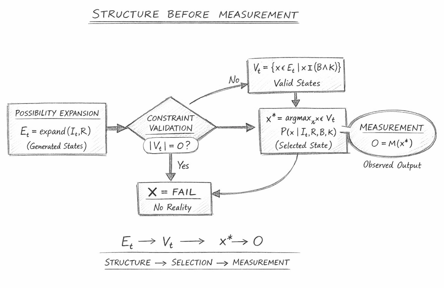
Structure Before Measurement — Execution Geometry

The diagram represents a directed constraint-resolution pipeline in which physical reality emerges only after structural validation, with measurement appearing strictly as a terminal operation.

It should be interpreted as a causal–logical flow, not a temporal cartoon.

1. Possibility Expansion — Pre-Physical State Generation

The leftmost block:

\[ E_t = \operatorname{expand}(I_t, R) \]

represents the generation of candidate configurations from the current information state under governing rules.

Scientifically, this corresponds to:

  • solution spaces of differential equations
  • quantum configuration spaces
  • phase space evolution in classical mechanics

However, the diagram makes an explicit distinction often left implicit:

Not all mathematically generated states are physically admissible.

Thus, this stage defines:

  • possibility space (superset)
  • not physical reality

2. Constraint Validation — Definition of Physical Admissibility

The central diamond:

\[ V_t = \{ x \in E_t \mid x \models (B \land K) \} \]

is the critical structural boundary of the entire system.

Here:

  • BB encodes boundary conditions (geometry, causality, interaction limits)
  • KK encodes invariants (conservation laws, symmetries, consistency rules)

This stage implements:

Physical law as a filtering operator, not a descriptive overlay.

Only states that satisfy all constraints survive.

Everything else is eliminated from physical consideration.

3. Null Condition — Structural Non-Existence

The branch:

\[ |V_t| = 0 \;\Rightarrow\; X = \text{FAIL} \]

represents a hard physical boundary:

  • No valid state exists
  • No continuation is possible
  • No measurement can occur

This must be interpreted as:

A system with no constraint-satisfying state has no physical reality.

This replaces vague notions such as “undefined” with a strict criterion:

Existence requires structural consistency

4. Valid State Set — Emergence of Physical Structure

If the constraint condition is satisfied, the system enters:

\[ V_t \neq \varnothing \]

This block represents:

  • the physically admissible state space
  • the set of all states that could exist under the laws of physics

At this stage:

  • reality is not yet singular
  • it is a structured set of valid possibilities

5. Selection — Resolution Within Structured Reality

The next block:

\[ x^* = \arg\max_{x \in V_t} P(x \mid I_t, R, B, K) \]

implements state resolution.

Scientifically, this corresponds to:

  • probabilistic selection in quantum systems
  • energy minimisation in thermodynamics
  • action extremisation in classical mechanics

The key constraint is:

Selection operates only within VtV_t, never outside it.

Thus:

  • randomness is bounded
  • determinism is preserved where applicable
  • no invalid state can ever be selected

6. Measurement — Terminal Projection

The final block:

\[ O = M(x^*) \]

represents measurement as a mapping from resolved structure to observable output.

Critically:

  • measurement occurs after structure is fully resolved
  • measurement does not influence validity
  • measurement does not generate the state

This directly contradicts interpretations such as the
Copenhagen interpretation, where measurement is often treated as:

  • collapsing an undefined system into reality

Instead, the diagram enforces:

Measurement is a readout of an already valid, selected state.

7. Global Flow — Structural Ordering

The bottom relation:

\[ E_t \to V_t \to x^* \to O \]

encodes the non-reversible ordering of the system:

  • 1. Generate possibilities
  • 2. Enforce constraints
  • 3. Resolve state
  • 4. Measure outcome

This ordering is fundamental:

  • It cannot be rearranged
  • It defines the direction of physical legitimacy

8. Structural Principle Encoded by the Diagram

The final statement:

Structure→Selection→Measurement

summarises the entire framework.

It encodes a strict hierarchy:

  • Structure defines what can exist
  • Selection determines what does exist
  • Measurement reveals what exists

9. Scientific Significance

This diagram implements a fundamental inversion of standard interpretation:

Traditional View

Measurement reveals or creates reality

This Framework
  • Reality must already be structurally valid
  • Measurement can only access that structure

Final Scientific Statement

The diagram is not illustrative — it is formal.

It encodes the necessary condition:

A system must first satisfy all structural constraints before it can exist,
and only then can it be measured.

Closing Insight

What appears as a simple flowchart is, in fact, a complete execution geometry of physical reality:

  • invalid structure → no existence
  • valid structure → selectable state
  • selected state → measurable outcome

And therefore:

Measurement is not the origin of reality —
it is the final interface with a structure that already exists.

Execution Guarantee Statement

Structural Necessity of Measurement

The preceding flow and its mathematical mappings establish a strict condition on all physically meaningful systems:

\[ V_t \neq \varnothing \;\Leftrightarrow\; \text{Measurement is defined} \]

and therefore:

\[ V_t = \varnothing \;\Longrightarrow\; \text{No observable reality exists} \]

This is not an interpretive statement — it is a logical requirement.

Formal Guarantee

For any system S=(I,R,B,K)S = (I, R, B, K):

\[ O \text{ exists} \;\Leftrightarrow\; \exists x \in E_t \;\text{such that}\; x \models (B \land K) \]

Thus:

  • Measurement requires a valid structural domain
  • Observables require constraint satisfaction prior to detection
  • No measurement process can operate outside VtV_t

Irreversibility of Ordering

The execution ordering:

\[ E_t \to V_t \to x^* \to O \]

is non-commutative.

Any attempt to reorder:

  • O→x∗O \rightarrow x^* (measurement before selection)
  • O→VtO \rightarrow V_t (measurement before validation)

results in:

Undefined operation

Physical Consequence

This enforces a universal constraint:

No theory can consistently treat measurement as fundamental
without implicitly assuming prior structure.

Thus:

  • Measurement-first ontologies are incomplete
  • Observer-dependent reality models are structurally underdefined
  • Physical law must act before observation, not after

Final Closure

\[ O = M\bigl(R(I) \mid (B, K)\bigr) \]

is not just a formulation — it is a boundary condition on reality itself.

Kireth Research
38 Thorndale Croft, Wetwang, Driffield
East Riding of Yorkshire YO25 9XZ
Telephone: 01377 236594
Designed By