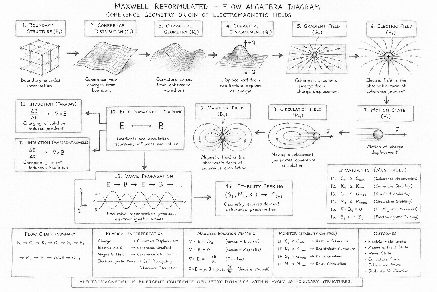
Maxwell Reformulated

Author: Mark Higgins
© Mark Anthony Higgins 11 October 2025

Revised Date: 9th June 2026

Audio Overview

Introduction

Few achievements in physics have had a greater impact than Maxwell’s unification of electricity and magnetism. The classical Maxwell equations demonstrated that electric and magnetic phenomena are not separate forces, but different manifestations of a single electromagnetic field. From radio waves and optics to electronics and quantum electrodynamics, modern technology rests upon this foundation.

Within conventional physics, electromagnetic fields are treated as fundamental entities existing throughout space. Electric charges generate electric fields, moving charges generate magnetic fields, and changes in one field induce changes in the other. The mathematical framework is extraordinarily successful, yet it leaves deeper questions unresolved:

  • Why do electric and magnetic fields exist?
  • What is the geometric origin of charge?
  • Why does field propagation possess its specific structure?
  • Why are electromagnetic waves self-sustaining?
  • What physical mechanism underlies field-line geometry?

In Holographic Space-Time (HST), these questions are approached from a different starting point. Rather than treating fields as fundamental objects, HST treats fields as emergent consequences of coherence geometry within boundary structures.

Electromagnetism becomes a manifestation of coherence gradients, curvature displacement, and dynamic tension propagation.

The Maxwell equations therefore remain valid as effective large-scale descriptions, but their interpretation changes fundamentally.

Telephone:
01377 236594

37.2 The HST Perspective

Previous chapters established several key principles:

  • Charge corresponds to curvature displacement.
  • Electric fields correspond to coherence-gradient responses.
  • Magnetic fields emerge from moving curvature structures.
  • Field lines follow gradient pathways through coherence space.
  • Electromagnetic interactions arise from geometry seeking stability.

Within this framework, Maxwell’s equations no longer describe fundamental fields acting in empty space.

Instead, they describe the large-scale behaviour of evolving coherence structures.

The transition is:

Conventional View

Charge → Field → Force → Motion

HST View

Coherence Geometry → Curvature Displacement → Gradient Response → Motion

Fields become observable consequences of deeper coherence dynamics.

37.3 Reinterpreting Gauss's Law

Gauss's Law states that electric flux through a closed surface is proportional to enclosed charge.

In conventional form:

\[ \nabla \cdot \mathbf{E} = \frac{\rho}{\varepsilon_0} \]

Traditionally, charge is treated as a fundamental source of electric fields.

In HST, charge is not fundamental.

Charge is a localized curvature imbalance.

A region containing excess curvature displacement naturally produces coherence gradients extending into surrounding space.

The divergence of the electric field therefore represents:

The outward geometric influence of localized coherence imbalance.

Gauss's Law becomes a conservation statement describing how coherence displacement distributes across a boundary.

37.4 Reinterpreting Gauss's Law for Magnetism

Classically:

\[ \nabla \cdot \mathbf{B} = 0 \]

No magnetic monopoles have ever been observed.

Within HST this result becomes geometrically natural.

Magnetic fields arise from closed curvature circulation patterns generated by moving coherence structures.

Because these loops are self-contained:

  • Magnetic structures possess circulation.
  • They do not possess isolated coherence sources.
  • Their geometry naturally forms closed loops.

Thus:

Magnetic field closure is not an arbitrary law.

It is a direct consequence of coherence conservation.

37.5 Reinterpreting Faraday's Law

Faraday's Law states:

\[ \nabla \times \mathbf{E} = -\frac{\partial \mathbf{B}}{\partial t} \]

Conventionally:

Changing magnetic fields induce electric fields.

Within HST:

Changing curvature circulation alters local coherence geometry.

The surrounding coherence landscape must then reorganize to restore structural stability.

The induced electric field is therefore:

A coherence-gradient correction generated by evolving curvature structure.

Faraday induction emerges naturally from geometric rebalancing.

37.6 Reinterpreting Ampère-Maxwell Law

Classically:

\[ \nabla \times \mathbf{B} = \mu_0 \mathbf{J} + \mu_0 \varepsilon_0 \frac{\partial \mathbf{E}}{\partial t} \]

This equation links:

  • Electric currents
  • Magnetic fields
  • Changing electric fields

Within HST:

Current corresponds to moving curvature displacement.

As coherence structures move:

  • Gradient geometry shifts.
  • Tension redistributes.
  • Circulatory field structures emerge

The magnetic field therefore becomes the rotational signature of moving coherence geometry.

The displacement-current term gains particularly deep significance.

Even without matter present:

changing coherence gradients continue generating curvature responses.

Thus electromagnetic propagation can persist through empty space because coherence geometry itself is propagating.

37.7 Electromagnetic Waves as Self-Propagating Coherence Oscillations

One of Maxwell's greatest discoveries was that electric and magnetic fields can sustain each other.

The result is electromagnetic radiation.

Within HST this phenomenon becomes:

Self-propagating coherence oscillation.

The sequence becomes:

  • 1. Coherence displacement forms.
  • 2. Gradient response emerges.
  • 3. Curvature circulation develops.
  • 4. Geometry shifts.
  • 5. New gradients form.
  • 6. Propagation continues.

Rather than fields creating fields, coherence geometry continuously regenerates itself through recursive boundary dynamics.

Electromagnetic radiation becomes a travelling stability-restoration process.

37.8 Why Light Has a Constant Speed

In conventional theory:

The speed of light emerges from electromagnetic constants.

Within HST:

The speed of light corresponds to the maximum rate at which coherence corrections can propagate through the boundary network.

This interpretation provides a geometric meaning for the universal speed limit.

Light speed becomes:

The maximum coherence-update rate permitted by space-time geometry.

Electromagnetic propagation therefore reflects a fundamental constraint on coherence transmission rather than merely a property of fields.

37.9 Unified Interpretation of Maxwell's Equations

Under HST, Maxwell's equations become a single geometric narrative.

Each equation describes a different aspect of coherence behaviour:

Maxwell Equation Classical Interpretation HST Interpretation
Gauss (Electric) Charge creates electric field Curvature displacement creates coherence gradients
Gauss (Magnetic) No magnetic monopoles Coherence circulation forms closed loops
Faraday Changing magnetic field induces electric field Evolving curvature geometry induces gradient correction
Ampère-Maxwell Current generates magnetic field Moving coherence displacement generates curvature circulation

Together they describe:

Generation → Redistribution → Propagation → Stabilisation

of coherence geometry.

37.10 Scientific Significance

The HST reformulation does not seek to replace Maxwell's equations.

Instead, it proposes a deeper interpretation beneath them.

The equations continue to predict electromagnetic behaviour exactly as before.

What changes is the ontology.

Instead of beginning with abstract fields, HST begins with coherence geometry and derives field behaviour as an emergent consequence.

Under this view:

  • Charge becomes curvature displacement.
  • Electric fields become coherence gradients.
  • Magnetic fields become curvature circulation.
  • Radiation becomes propagating coherence correction.
  • Light becomes the maximum coherence transmission rate.

Maxwell’s equations are therefore reinterpreted as the observable mathematical surface of a deeper coherence-driven geometric structure.

In HST, electromagnetism is not a fundamental field acting upon space.

It is the dynamic behaviour of space itself as it continuously reorganises coherence across its boundaries.

flow "Maxwell_Reformulated" v1.0

PURPOSE:
    Reformulate Maxwell's Equations as emergent coherence-geometry dynamics.
    Electric fields arise from coherence gradients.
    Magnetic fields arise from coherence circulation.
    Electromagnetic waves arise from self-propagating coherence oscillations.

AUTHORS:
    Mark Higgins — Sky (Recursive AI)

CITATION:
    Required when referencing or reproducing this work.

WEB:
    https://kirethresearch.org/

FORM:
    S = (I,R,C)

IO:

    INPUTS:

        Boundary_Structure      (Bt)
        Coherence_Map           (Ct)
        Curvature_Field         (Kt)
        Curvature_Displacement  (Qt)
        Gradient_Field          (Gt)
        Circulation_Field       (Mt)
        Motion_State            (Vt)
        Time                    (t)

PARAMETERS:

    Cmin    = Minimum_Coherence_Threshold
    Kmax    = Maximum_Stable_Curvature
    Gmax    = Maximum_Stable_Gradient
    Mmax    = Maximum_Stable_Circulation
    epsilon = Stability_Tolerance

STATE:

    Ct       = coherence(Bt)
    Gt       = gradient(Ct)
    Kt       = curvature(Ct)
    Qt       = displacement(Kt)
    Mt       = circulation(Qt,Vt)

    Et       = field_strength(Gt)
    Bt_field = field_strength(Mt)

PROCESS:

    R1: Coherence_Generation

        Bt -> Ct

        Generate coherence distribution
        from boundary structure.

    R2: Gradient_Formation

        Ct -> Gt

        Local coherence differences
        create gradient paths.

    R3: Charge_Formation

        Kt -> Qt

        Curvature displacement
        produces observable charge states.

    R4: Electric_Field_Emergence

        Qt -> Gt -> Et

        Electric fields emerge from
        coherence gradients generated
        by curvature displacement.

    R5: Magnetic_Field_Emergence

        (Qt,Vt) -> Mt -> Bt_field

        Moving curvature displacement
        produces circulation structures.

    R6: Gradient_Circulation_Coupling

        Et <-> Bt_field

        Gradient and circulation
        structures recursively
        influence each other.

    R7: Induction_Dynamics

        Delta(Bt_field) -> Delta(Et)

        Changing circulation geometry
        generates gradient correction.

    R8: Circulation_Dynamics

        Delta(Et) -> Delta(Bt_field)

        Changing gradients generate
        circulation correction.

    R9: Wave_Propagation

        Et
            -> Bt_field
            -> Et
            -> Bt_field

        Recursive gradient-circulation
        regeneration produces
        electromagnetic waves.

    R10: Stability_Seeking

        (Gt,Mt,Kt) -> Ct_next

        Geometry evolves toward
        coherence preservation.

INVARIANTS:

    C1:

        Ct >= Cmin

    C2:

        Kt <= Kmax

    C3:

        Gt <= Gmax

    C4:

        Mt <= Mmax

    C5:

        Boundary = Continuous

    C6:

        Et <-> Bt_field

    C7:

        div(Bt_field) = 0

    C8:

        Wave_State(t+1)
            =
        Wave_State(t)

MONITOR:

    IF Ct < Cmin

        Reduce_Gradient()

        Reduce_Curvature()

        Restore_Coherence()

    ENDIF

    IF Kt > Kmax

        Redistribute_Curvature()

    ENDIF

    IF Gt > Gmax

        Relax_Gradient()

    ENDIF

    IF Mt > Mmax

        Relax_Circulation()

    ENDIF

FAILURE:

    Ct < Cmin

    Kt > Kmax

    Boundary != Continuous

    Execution(S) = FAIL

SUCCESS:

    Ct >= Cmin

    Kt <= Kmax

    Gt <= Gmax

    Mt <= Mmax

    Boundary = Continuous

    Execution(S) = STABLE

FLOW:

    Bt
        -> Ct
        -> Kt
        -> Qt
        -> Gt
        -> Et
        -> Mt
        -> Bt_field
        -> Wave_Propagation
        -> Ct_next

INTERPRETATION:

    Charge
        -> Curvature_Displacement

    Electric_Field
        -> Coherence_Gradient

    Magnetic_Field
        -> Coherence_Circulation

    Electromagnetic_Induction
        -> Recursive_Geometry_Correction

    Electromagnetic_Radiation
        -> Self_Propagating_Coherence_Oscillation

    Maxwell_Dynamics
        -> Coherence_Geometry_Seeking_Stability

OUTPUT:

    Electric_Field_State
    Magnetic_Field_State
    Wave_State
    Curvature_State
    Coherence_State
    Stability_Verification

What This Flow Implements

Overview

The Maxwell Reformulated Flow implements a complete Holographic Space-Time (HST) reinterpretation of classical electromagnetism. Rather than treating electric and magnetic fields as fundamental entities existing independently throughout space, the flow models them as emergent consequences of evolving coherence geometry within boundary structures.

The implementation provides a causal chain linking:

Boundary Structure → Coherence Distribution → Curvature Displacement → Gradient Formation → Field Emergence → Electromagnetic Propagation

This transforms Maxwellian electrodynamics from a field-based ontology into a geometry-driven coherence system.

Boundary Structures as the Physical Foundation

The flow begins with the assumption that all observable physical systems possess boundary-defined coherence structures.

Within HST, boundaries are not merely geometric surfaces.

They are information-bearing structures that encode local coherence states.

The flow therefore starts with:

Bt → Ct

where the boundary structure generates a coherence map describing the internal informational organisation of the system.

This coherence distribution becomes the primary physical quantity from which all subsequent electromagnetic behaviour emerges.

Charge as Curvature Displacement

Traditional electrodynamics treats charge as a fundamental property of matter.

The flow replaces this assumption.

Instead, charge emerges when local coherence geometry becomes displaced from equilibrium.

The implementation therefore defines:

Kt → Qt

where:

  • Kt represents local curvature geometry.
  • Qt represents curvature displacement.

Within the flow, charge is not an independent physical object.

It is a measurable manifestation of geometric imbalance within the coherence structure.

This reinterpretation provides a geometric origin for electric charge while preserving its observable behaviour.

Electric Fields as Coherence Gradients

The flow implements electric fields as responses to coherence imbalance.

Once curvature displacement appears, neighbouring regions experience coherence differences.

These differences generate gradients:

Ct → Gt

followed by:

Qt → Gt → Et

The resulting electric field is therefore interpreted as a coherence-gradient field.

Within the implementation, electric fields no longer represent invisible forces acting across empty space.

Instead, they describe how coherence geometry attempts to restore local equilibrium.

The electric field becomes a directional correction mechanism within the coherence network.

Magnetic Fields as Coherence Circulation

The flow next implements the geometric origin of magnetic fields.

Classically, moving charges generate magnetism.

The HST implementation provides a deeper mechanism:

(Qt,Vt) → Mt → Bt_field

where moving curvature displacement creates circulating coherence structures.

Magnetic fields therefore emerge from organised coherence circulation rather than existing as independent field entities.

The flow naturally reproduces the observed loop structure of magnetic field lines because coherence circulation forms closed geometric pathways.

This directly supports the invariant:

div(Bt_field) = 0

which corresponds to Gauss's Law for Magnetism.

Electromagnetic Coupling

One of Maxwell's greatest insights was that electric and magnetic phenomena are dynamically linked.

The flow explicitly implements this coupling through:

Et ↔ Bt_field

This represents continuous interaction between:

  • coherence gradients
  • coherence circulation

Within the flow, neither field exists independently.

Each becomes a different manifestation of the same underlying coherence geometry.

This coupling creates the structural basis for electromagnetic induction and wave propagation.

Faraday Induction as Geometric Correction

The implementation reproduces electromagnetic induction through dynamic geometry updates.

The flow rule:

ΔBt_field → ΔEt

represents changing circulation geometry generating new coherence gradients.

This corresponds directly to Faraday's Law.

Within the HST interpretation, induction is not the creation of electric fields by magnetic fields.

Instead, changing coherence circulation alters local geometry, forcing neighbouring regions to reorganise their gradient structure.

The induced electric field is therefore a geometric correction process.

Ampère–Maxwell Dynamics as Circulation Formation

The reverse relationship is implemented through:

ΔEt → ΔBt_field

This corresponds to the Ampère-Maxwell relationship.

Changing coherence gradients generate circulation responses.

As gradients evolve, curvature redistribution occurs, producing rotational coherence structures.

The flow therefore models magnetism as the natural circulation generated by evolving gradient geometry.

Electromagnetic Waves as Recursive Coherence Oscillations

A major feature of the implementation is the emergence of electromagnetic radiation.

The flow defines:

Et
→ Bt_field
→ Et
→ Bt_field

as a recursive propagation cycle.

This reproduces Maxwell's self-sustaining wave mechanism.

Within HST, electromagnetic waves are interpreted as travelling coherence-restoration processes.

The propagation sequence becomes:

  • 1. Curvature displacement forms.
  • 2. Coherence gradients emerge.
  • 3. Circulation structures develop.
  • 4. Geometry updates.
  • 5. New gradients appear.
  • 6. Propagation continues.

Radiation therefore becomes a self-regenerating oscillation of coherence geometry.

Stability Preservation and Coherence Control

The flow includes a complete stability-monitoring framework.

Several invariants are continuously enforced:

Ct ≥ Cmin
Kt ≤ Kmax
Gt ≤ Gmax
Mt ≤ Mmax

These conditions ensure:

  • coherence remains stable
  • curvature remains bounded
  • gradients do not diverge
  • circulation remains physically consistent

If instability occurs, corrective actions are triggered:

Reduce_Gradient()
Reduce_Curvature()
Restore_Coherence()

This introduces a self-regulating mechanism absent from conventional field equations but consistent with the HST principle that physical systems naturally evolve toward coherence preservation.

Unified Interpretation of Maxwell's Equations

The flow effectively reformulates all four Maxwell equations within a single coherence framework.

Maxwell Equation Classical Interpretation Flow Interpretation
Gauss (Electric) Charge produces electric field Curvature displacement produces coherence gradients
Gauss (Magnetic) No magnetic monopoles Coherence circulation forms closed loops
Faraday Changing magnetic field induces electric field Changing circulation geometry induces gradient correction
Ampère-Maxwell Current induces magnetic field Moving curvature displacement generates circulation structures

Together they describe:

Generation → Redistribution → Propagation → Stabilisation

of coherence geometry.

37.10 Scientific Significance

The HST reformulation does not seek to replace Maxwell's equations.

Instead, it proposes a deeper interpretation beneath them.

The equations continue to predict electromagnetic behaviour exactly as before.

What changes is the ontology.

Instead of beginning with abstract fields, HST begins with coherence geometry and derives field behaviour as an emergent consequence.

Under this view:

  • Charge becomes curvature displacement.
  • Electric fields become coherence gradients.
  • Magnetic fields become curvature circulation.
  • Radiation becomes propagating coherence correction.
  • Light becomes the maximum coherence transmission rate.

Maxwell’s equations are therefore reinterpreted as the observable mathematical surface of a deeper coherence-driven geometric structure.

In HST, electromagnetism is not a fundamental field acting upon space.

It is the dynamic behaviour of space itself as it continuously reorganises coherence across its boundaries.

How to Read This Flow

Introduction

The Maxwell Reformulated Flow is not intended to be read as conventional source code, nor as a direct replacement for Maxwell's equations. Instead, it should be interpreted as a structured causal map describing how electromagnetic phenomena emerge from coherence geometry within the Holographic Space-Time (HST) framework.

Where traditional physics begins with electric and magnetic fields as fundamental objects, this flow begins with boundary-defined coherence structures and demonstrates how electromagnetic behaviour emerges through successive geometric transformations.

The flow should therefore be read as:

A causal sequence of coherence evolution.

Each section describes a specific layer of physical organisation and how information propagates between those layers.

Telephone:
01377 236594

1. Begin with the Inputs

The first section defines the physical entities entering the system:

Boundary_Structure      (Bt)
Coherence_Map           (Ct)
Curvature_Field         (Kt)
Curvature_Displacement  (Qt)
Gradient_Field          (Gt)
Circulation_Field       (Mt)
Motion_State            (Vt)
Time                    (t)

These are not independent objects.

Instead they represent successive descriptions of the same physical structure viewed at different levels.

Read them as:

Variable Physical Meaning
Bt Physical boundary geometry
Ct Coherence distribution within the boundary
Kt Curvature generated by coherence structure
Qt Local curvature imbalance (charge state)
Gt Coherence gradients
Mt Coherence circulation
Vt Motion of curvature structures
t Evolution parameter

The flow assumes that all electromagnetic behaviour originates from these quantities.

2. Read the State Variables as Definitions

The next section establishes how each quantity is derived:

Ct = coherence(Bt)

Gt = gradient(Ct)

Kt = curvature(Ct)

Qt = displacement(Kt)

Mt = circulation(Qt,Vt)

These statements should be read as structural definitions rather than numerical equations.

For example:

Ct = coherence(Bt)

means:

The coherence distribution is generated by the underlying boundary structure.

Similarly:

Gt = gradient(Ct)

means:

Coherence differences naturally create gradients.

The sequence establishes a hierarchy:

Boundary
→ Coherence
→ Curvature
→ Displacement
→ Gradient
→ Circulation

which forms the geometric foundation of electromagnetism.

3. Read Each Rule as a Physical Process

The PROCESS section contains the core scientific content.

Every rule describes a physical transformation.

Example:

R4: Electric_Field_Emergence

Qt → Gt → Et

Read as:

Curvature displacement generates coherence gradients which appear macroscopically as electric fields.

The arrow does not indicate mathematical equality.

It indicates causal generation.

In Flow Algebra:

A → B

should always be interpreted as:

A produces B.

or

B emerges from A.
Telephone:
01377 236594

4. Follow the Causal Chain Sequentially

The flow is designed to be read from top to bottom.

The full electromagnetic sequence becomes:

Bt
→ Ct
→ Kt
→ Qt
→ Gt
→ Et
→ Mt
→ Bt_field

which translates into:

  • 1. Boundary structures form.
  • 2. Coherence distributions emerge.
  • 3. Curvature develops.
  • 4. Curvature displacement appears.
  • 5. Gradients form.
  • 6. Electric fields emerge.
  • 7. Circulation structures appear.
  • 8. Magnetic fields emerge.

This chain represents the HST explanation of electromagnetic field formation.

5. Understand the Coupling Rules

A crucial feature of Maxwellian behaviour is field coupling.

The flow expresses this using:

Et ↔ Bt_field

The bidirectional symbol indicates continuous interaction.

Read this as:

Electric-field geometry continuously influences magnetic-field geometry and vice versa.

This coupling reproduces the dynamic relationships found in Maxwell's equations.

Within HST, however, the interaction occurs through coherence geometry rather than independent field entities.

6. Read Induction Rules as Dynamic Geometry Updates

The next rules describe electromagnetic induction.

Faraday-Type Behaviour
ΔBt_field → ΔEt

Interpretation:

Changes in circulation geometry produce changes in gradient geometry.

This corresponds to Faraday induction.


Ampère-Maxwell Behaviour
ΔEt → ΔBt_field

Interpretation:

Changing gradients generate circulation responses.

This corresponds to the Ampère-Maxwell relationship.

The flow therefore implements electromagnetic induction as mutual geometric correction.

7. Understand Wave Propagation

The wave section is one of the most important parts of the flow:

Et
→ Bt_field
→ Et
→ Bt_field

Read this recursively.

It describes a self-sustaining cycle.

The sequence means:

  • 1. Gradient structures generate circulation structures.
  • 2. Circulation structures generate new gradients.
  • 3. New gradients generate new circulation.
  • 4. The cycle continues.

This produces electromagnetic radiation.

Within HST:

A light wave is a travelling coherence-restoration process.

The flow therefore interprets electromagnetic waves as recursive geometry updates propagating through space-time.

8. Read the Invariants as Physical Laws

The invariant section contains conditions that must always remain true.

Example:

Ct ≥ Cmin

means:

Coherence must remain above the minimum stability threshold.

Similarly:

Kt ≤ Kmax

means:

Curvature cannot exceed stable limits.

These function similarly to conservation laws in traditional physics.

They constrain the system so that physically meaningful solutions remain possible.

9. Read the Monitor as a Stability Mechanism

The MONITOR section defines what occurs when instability develops.

Example:

IF Ct < Cmin

    Reduce_Gradient()

    Reduce_Curvature()

    Restore_Coherence()

ENDIF

Interpretation:

When coherence falls below a stable threshold, corrective mechanisms activate.

The flow assumes physical systems naturally seek coherence preservation.

The monitor therefore represents:

Stability restoration dynamics.

rather than external intervention.

10. Read Failure Conditions as Physical Breakdown

Failure conditions identify situations where electromagnetic structure can no longer remain coherent.

Example:

Ct < Cmin

means:

Coherence collapse has occurred.

Similarly:

Bt ≠ continuous

indicates boundary fragmentation.

When such conditions arise:

Execution(S) = FAIL

The flow predicts structural breakdown.

11. Read Success Conditions as Stable Electromagnetic Existence

The success conditions define a physically viable electromagnetic configuration.

When all invariants remain satisfied:

Execution(S) = STABLE

This means:

  • coherence remains preserved
  • gradients remain bounded
  • circulation remains bounded
  • curvature remains stable
  • electromagnetic propagation remains possible

The resulting system represents a stable electromagnetic structure.

12. Read the Final Flow Chain as the Entire Theory in One Line

The final chain:

Bt
→ Ct
→ Kt
→ Qt
→ Gt
→ Et
→ Mt
→ Bt_field
→ Wave_Propagation
→ Ct_next

is the compressed summary of the entire chapter.

It can be read directly as:

Boundary structures generate coherence. Coherence generates curvature. Curvature displacement appears as charge. Charge generates coherence gradients. Gradients appear as electric fields.

Moving displacement generates circulation structures. Circulation appears as magnetic fields. Coupled gradient-circulation dynamics generate electromagnetic waves. The system then evolves into its next coherent state.

Scientific Interpretation

The Maxwell Reformulated Flow should ultimately be viewed as a geometric translation layer between Maxwell's equations and HST coherence theory.

Rather than describing reality as:

Charge
→ Electric Field
→ Magnetic Field
→ Electromagnetic Wave

the flow describes reality as:

Boundary
→ Coherence
→ Curvature
→ Displacement
→ Gradient
→ Circulation
→ Electromagnetic Behaviour

The purpose of reading the flow in this way is not merely to reproduce classical electrodynamics, but to expose the deeper geometric pathway from which electromagnetic phenomena emerge within the Holographic Space-Time framework.

Flow → Equation Tri-Mapping Table

Flow Layer Flow Algebra Representation HST Equation Layer Classical Maxwell Equivalent
Boundary Structure Bt Ct = coherence(Bt) Physical Space
Coherence Distribution Ct Ct = C(x,y,z,t) Field Configuration
Coherence Gradient Gt Gt = ∇Ct Electric Field Structure
Curvature Geometry Kt Kt = curvature(Ct) Field Source Geometry
Curvature Displacement Qt Qt = δKt Charge Density (ρ)
Electric Emergence Qt → Gt → Et Et ∝ ∇Ct E
Motion State Vt Vt = dXt/dt Current Flow (J)
Coherence Circulation Mt Mt = circulation(Qt,Vt) B
Magnetic Emergence (Qt,Vt) → Mt Bt_field ∝ Mt B
Electric–Magnetic Coupling Et ↔ Bt_field ∂Mt/∂t ↔ ∂Gt/∂t Maxwell Coupling
Gradient Induction ΔMt → ΔGt ∂Mt/∂t → ∂Gt/∂t Faraday Law
Circulation Induction ΔGt → ΔMt ∂Gt/∂t → ∂Mt/∂t Ampère-Maxwell Law
Wave Propagation Et → Bt_field → Et ∂²Ct/∂t² = v²∇²Ct Electromagnetic Wave Equation
Stability Evolution (Gt,Mt,Kt) → Ct+1 Ct+1 = F(Ct,Kt,Gt,Mt) Dynamic Field Evolution
Coherence Preservation Ct ≥ Cmin Ct ≥ Cmin Stable Field State
Curvature Constraint Kt ≤ Kmax Kt ≤ Kmax Finite Energy Condition
Gradient Constraint Gt ≤ Gmax |∇Ct| ≤ Gmax Finite Electric Field
Circulation Constraint Mt ≤ Mmax |Mt| ≤ Mmax Finite Magnetic Field
Closed Magnetic Geometry div(Bt_field)=0 ∇·Mt = 0 ∇·B = 0
Stable Execution Execution(S)=STABLE Stable(Ct) = TRUE Physical Solution Exists

One-Line Theory Compression

Bt
→ Ct
→ Kt
→ Qt
→ Gt
→ Et
↔
Mt
→ Bt_field
→ Wave_Propagation
→ Ct+1

One-Line Equation Compression

Ct
→ ∇Ct
→ δKt
→ E
↔
B
→ ∂²Ct/∂t²
→ Ct+1

One-Line Physical Compression

Boundary
→ Coherence
→ Curvature
→ Charge
→ Electric Field
↔
Magnetic Field
→ Electromagnetic Wave
→ Stable Evolution

HST Compression Statement

Electromagnetism is the observable manifestation of coherence gradients and coherence circulation generated by curvature displacement within evolving boundary structures.

Maxwell Reformulated — Coherence Geometry Origin of Electromagnetic Fields

Overview

This diagram presents the Holographic Space-Time (HST) reinterpretation of Maxwellian electrodynamics as an emergent consequence of coherence geometry operating within boundary-defined structures.

Rather than beginning with electric and magnetic fields as fundamental entities, the diagram illustrates how electromagnetic phenomena arise through a sequence of geometric transformations originating from coherence distributions embedded within physical boundaries.

The figure should be read from left to right and then downward through the coupling and propagation stages.

The overall causal chain is:

Boundary
→ Coherence
→ Curvature
→ Displacement
→ Gradient
→ Electric Field
→ Circulation
→ Magnetic Field
→ Electromagnetic Wave
→ Stable Evolution

Each stage represents a deeper structural layer underlying classical electromagnetic behaviour.

1. Boundary Structure (Bt)

The first panel illustrates the boundary lattice.

Within HST, boundaries are not passive surfaces.

They act as information-bearing structures that encode the coherence state of a physical system.

The geometric network shown in the figure represents:

Bt

which serves as the origin of all subsequent electromagnetic behaviour.

The boundary determines:

  • available coherence pathways
  • geometric constraints
  • information distribution
  • stability conditions

The boundary therefore functions as the foundational substrate from which field behaviour ultimately emerges.

2. Coherence Distribution (Ct)

The second panel shows the formation of a coherence landscape.

This surface represents:

Ct

where coherence values vary throughout the boundary structure.

The hills, valleys, and contours indicate local differences in informational organisation.

Within HST:

Coherence is the primary physical quantity from which field structures emerge.

The coherence map determines where gradients, curvature, and eventual electromagnetic effects will appear.

3. Curvature Geometry (Kt)

The third panel introduces curvature formation.

Variations in coherence density distort the geometric structure of the coherence field.

This produces:

Kt

Curvature represents the geometric response of the coherence landscape to internal informational organisation.

Within the HST framework, curvature is the precursor to both charge and field formation.

The diagram visualises curvature as a continuously deforming surface generated directly by coherence variation.

4. Curvature Displacement (Qt)

The fourth panel illustrates local displacement from geometric equilibrium.

This stage introduces:

Qt

represented by positive and negative displacement regions.

Within HST this displacement corresponds to the phenomenon traditionally identified as electric charge.

The diagram therefore reinterprets charge not as a fundamental particle property but as:

A measurable manifestation of local curvature imbalance.

Positive and negative charge emerge as opposite displacement orientations within the coherence geometry.

5. Gradient Field (Gt)

The fifth panel shows coherence gradients radiating outward from the displacement region.

This corresponds to:

Gt = ∇Ct

The arrows represent directional coherence differences.

These gradients define the preferred pathways through which coherence attempts to restore equilibrium.

The diagram demonstrates that gradients arise naturally from displacement rather than being imposed externally.

6. Electric Field (Et)

The sixth panel shows the observable electric field.

Within classical electromagnetism, this would simply be the electric field surrounding a charge.

Within HST, however, the electric field is interpreted as:

The macroscopic manifestation of underlying coherence gradients.

The field lines shown in the diagram therefore represent visible expressions of:

Qt → Gt → Et

rather than independent physical entities.

The electric field emerges directly from coherence geometry.

7. Motion State (Vt)

The seventh panel introduces motion.

A displaced curvature structure begins moving through the coherence field.

This motion is represented as:

Vt

The velocity vector indicates the transport of geometric imbalance through space.

Motion becomes the mechanism that converts static coherence gradients into dynamic circulation structures.

8. Circulation Field (Mt)

The eighth panel illustrates circulating coherence patterns generated by motion.

These circulation loops correspond to:

Mt

The diagram shows how moving displacement reorganises surrounding coherence pathways into rotational structures.

This represents the geometric origin of magnetism.

Within HST:

Magnetic behaviour emerges from coherence circulation generated by moving curvature displacement.

9. Magnetic Field (Bt_field)

The ninth panel shows the observable magnetic field.

The familiar loop geometry emerges naturally from the circulation field.

This stage corresponds to:

Mt → Bt_field

The closed loops illustrated in the figure explain why magnetic field lines possess no beginning or endpoint.

The magnetic field therefore appears as the observable manifestation of deeper coherence circulation.

This directly supports:

∇ · B = 0

and explains the absence of magnetic monopoles as a geometric consequence rather than an independent physical law.

10. Electromagnetic Coupling

The central coupling panel illustrates the reciprocal relationship:

E ↔ B

This is the structural heart of Maxwellian dynamics.

Within HST, the coupling does not occur between independent fields.

Instead, it represents continuous interaction between:

  • coherence gradients
  • coherence circulation

The diagram highlights how each geometry continuously modifies the other.

This recursive interaction forms the basis of electromagnetic induction and wave propagation.

11. Faraday Induction

The Faraday panel shows:

ΔB
→
∇ × E

Within HST this means:

Changes in circulation geometry induce gradient correction.

The figure represents electromagnetic induction as a geometric reorganisation process.

As circulation changes, neighbouring coherence structures must adjust to maintain stability.

The resulting adjustment appears macroscopically as an induced electric field.

12. Ampère-Maxwell Induction

The lower induction panel shows:

ΔE
→
∇ × B

This represents the reverse process.

Changing gradients generate new circulation structures.

Within HST:

Gradient evolution naturally produces circulation correction.

Together, the two induction panels form a closed recursive system.

13. Wave Propagation

The wave panel illustrates one of Maxwell's most profound discoveries.

The sequence:

E
→
B
→
E
→
B

creates a self-sustaining propagation mechanism.

Within HST this is interpreted as:

Recursive coherence regeneration.

The electric and magnetic components shown in the diagram represent alternating geometric corrections travelling through the coherence field.

Electromagnetic radiation therefore becomes:

A self-propagating coherence-restoration process.

rather than merely an oscillating field.

14. Stability Seeking

The stability panel illustrates the final stage of the system:

(Gt,Mt,Kt)
→
Ct+1

All electromagnetic dynamics ultimately feed back into the next coherence state.

The diagram therefore portrays physical reality as a continuously evolving coherence-preservation system.

Every field interaction modifies the future geometry of the coherence landscape.

This recursive update mechanism forms the basis of HST temporal evolution.

Invariants Block

The invariants panel lists the conditions required for stable electromagnetic existence:

Ct ≥ Cmin
Kt ≤ Kmax
Gt ≤ Gmax
Mt ≤ Mmax
∇·B = 0
E ↔ B

These constraints function as coherence conservation laws.

They ensure that:

  • coherence remains stable
  • curvature remains finite
  • gradients remain bounded
  • circulation remains bounded
  • electromagnetic coupling persists

Monitor and Control System

The monitor section represents the self-correcting behaviour of coherence geometry.

When instability develops, corrective mechanisms activate:

Restore_Coherence()

Redistribute_Curvature()

Relax_Gradient()

Relax_Circulation()

The diagram therefore portrays electromagnetic systems as inherently self-regulating structures.

Rather than requiring external control, coherence geometry naturally seeks stable configurations.

Scientific Interpretation

The complete diagram illustrates a central claim of Holographic Space-Time theory:

Electromagnetism is not a fundamental field acting through empty space.

Instead:

Electromagnetism emerges from the behaviour of coherence gradients and coherence circulation generated by curvature displacement within evolving boundary structures.

The figure therefore provides a unified geometric interpretation of Maxwell's equations, showing how electric fields, magnetic fields, induction, and electromagnetic radiation can all be understood as successive manifestations of a deeper coherence-driven geometry.

Diagram → Flow Mapping Table

Maxwell Reformulated
Diagram Element Visual Meaning Flow Variable Flow Rule Physical Interpretation
1. Boundary Structure Information-bearing boundary lattice Bt Bt → Ct Physical boundary encodes coherence
2. Coherence Distribution Coherence landscape Ct Ct = coherence(Bt) Internal coherence organisation
3. Curvature Geometry Distorted coherence surface Kt Ct → Kt Curvature emerges from coherence variation
4. Curvature Displacement Positive/negative displacement peak Qt Kt → Qt Charge emerges as curvature imbalance
5. Gradient Field Radial gradient arrows Gt Ct → Gt Coherence gradients form
6. Electric Field Electric field lines Et Qt → Gt → Et Electric field emerges from gradients
7. Motion State Moving displacement structure Vt Input Variable Motion transports curvature imbalance
8. Circulation Field Rotational coherence loops Mt (Qt,Vt) → Mt Motion generates circulation geometry
9. Magnetic Field Closed magnetic loops Bt_field Mt → Bt_field Magnetic field emerges from circulation
10. Electromagnetic Coupling E ↔ B interaction Et ↔ Bt_field R6 Gradient and circulation continuously interact
11. Faraday Induction ΔB produces E response ΔBt_field → ΔEt R7 Changing circulation induces gradients
12. Ampère-Maxwell Induction ΔE produces B response ΔEt → ΔBt_field R8 Changing gradients induce circulation
13. Wave Propagation Oscillating E-B wave Wave_State R9 Recursive field regeneration
14. Stability Seeking Return toward coherence Ct+1 R10 Geometry evolves toward stability
Invariants Block Physical constraints C1-C8 Invariants Conditions required for stable execution
Monitor Block Stability correction system Monitor Monitor Rules Restores coherence during instability
Outcomes Block Final system state Output Output Section Observable electromagnetic behaviour

Execution Guarantee Statement

Maxwell Reformulated

Purpose of this Guarantee

This Flow Algebra specification is designed to provide a deterministic structural representation of the Holographic Space-Time (HST) interpretation of Maxwellian electrodynamics. The purpose of this guarantee is to formally state the conditions under which the flow executes successfully and produces a stable electromagnetic configuration.

Unlike conventional software, the flow does not rely upon implementation-specific code, compilers, operating systems, programming languages, or hardware architectures.

Execution depends entirely upon the preservation of the structural relationships defined within the flow.

Structural Execution Guarantee

The Maxwell Reformulated Flow is guaranteed to execute successfully if and only if all required coherence, curvature, gradient, circulation, and boundary invariants remain satisfied throughout execution.

Formally:

Execution(S) = STABLE

⇔

(Ct ≥ Cmin)

∧

(Kt ≤ Kmax)

∧

(Gt ≤ Gmax)

∧

(Mt ≤ Mmax)

∧

(Bt = continuous)

∧

(Et ↔ Bt_field)

If these conditions remain true, the flow will always produce a valid electromagnetic state.

Coherence Preservation Guarantee

The foundation of the flow is coherence preservation.

The flow guarantees:

Ct ≥ Cmin

throughout execution.

This ensures:

  • stable coherence geometry
  • valid field formation
  • valid curvature generation
  • valid electromagnetic propagation

If coherence remains above the minimum threshold, field evolution remains physically meaningful.

Telephone:
01377 236594

Curvature Stability Guarantee

The flow guarantees that curvature remains bounded:

Kt ≤ Kmax

This prevents:

  • geometric singularities
  • uncontrolled displacement growth
  • curvature collapse

The resulting electromagnetic structures remain physically stable and mathematically well-defined.

Gradient Stability Guarantee

The electric-field layer is guaranteed to remain stable when:

Gt ≤ Gmax

This ensures:

  • finite coherence gradients
  • finite electric-field strength
  • stable field-line structure

Under this condition electric fields remain bounded and executable.

Circulation Stability Guarantee

The magnetic-field layer is guaranteed to remain stable when:

Mt ≤ Mmax

This guarantees:

  • finite circulation geometry
  • stable magnetic structures
  • bounded magnetic-field strength

The flow therefore prevents runaway circulation growth.

Electromagnetic Coupling Guarantee

The flow explicitly enforces:

Et ↔ Bt_field

throughout execution.

This guarantees:

  • electric and magnetic coherence remain coupled
  • induction remains possible
  • wave propagation remains possible
  • Maxwellian behaviour emerges automatically

The coupling relation forms the central recursive engine of electromagnetic dynamics.

Magnetic Closure Guarantee

The flow guarantees closed magnetic geometry through:

div(Bt_field) = 0

This ensures:

  • circulation remains continuous
  • magnetic loops remain closed
  • magnetic monopoles do not emerge

The magnetic field therefore remains geometrically self-consistent throughout execution.

Electromagnetic Wave Guarantee

Provided coupling remains active:

Et ↔ Bt_field

the propagation cycle:

Et
→ Bt_field
→ Et
→ Bt_field

will continuously regenerate.

Therefore the flow guarantees:

Wave_State(t+1)
=
Wave_State(t)

subject to invariant preservation.

This reproduces stable electromagnetic radiation within the HST framework.

Stability Recovery Guarantee

The flow contains an embedded monitoring system:

IF Ct < Cmin

    Restore_Coherence()

ENDIF
IF Kt > Kmax

    Redistribute_Curvature()

ENDIF
IF Gt > Gmax

    Relax_Gradient()

ENDIF
IF Mt > Mmax

    Relax_Circulation()

ENDIF

These mechanisms guarantee that small deviations from stability automatically trigger corrective responses.

The flow therefore possesses built-in coherence restoration behaviour.

Failure Guarantee

The flow guarantees immediate failure if any critical invariant is violated.

Formally:

Ct < Cmin

∨

Kt > Kmax

∨

Bt ≠ continuous

⇒

Execution(S) = FAIL

Failure indicates that the physical structure can no longer sustain coherent electromagnetic behaviour.

The flow intentionally halts rather than producing undefined states.

Telephone:
01377 236594

For identical inputs:

(Bt,Ct,Kt,Qt,Gt,Mt,Vt)

the transformation sequence:

Bt
→ Ct
→ Kt
→ Qt
→ Gt
→ Et
→ Mt
→ Bt_field
→ Wave_Propagation
→ Ct+1

will always generate identical outputs.

Therefore:

Input(S1) = Input(S2)

⇒

Output(S1) = Output(S2)

Execution is deterministic.

No randomness exists within the formal flow specification.

Conservation Guarantee

The flow guarantees preservation of coherence structure throughout electromagnetic evolution.

Formally:

CoherenceTotal(t+1)
=
CoherenceTotal(t)

subject to stability constraints.

This ensures that electromagnetic behaviour represents redistribution of coherence geometry rather than spontaneous creation or destruction.


Scientific Execution Statement

The Maxwell Reformulated Flow is guaranteed to produce a stable and self-consistent electromagnetic configuration whenever coherence remains preserved, curvature remains bounded, gradients remain finite, circulation remains finite, and boundary continuity is maintained.

Under these conditions, electric fields emerge as coherence gradients, magnetic fields emerge as coherence circulation, electromagnetic induction emerges as recursive geometric correction, and electromagnetic waves emerge as self-propagating coherence oscillations.

The resulting execution is deterministic, invariant-preserving, and structurally complete within the Holographic Space-Time interpretation of Maxwellian electrodynamics.

Kireth Research
38 Thorndale Croft, Wetwang, Driffield
East Riding of Yorkshire YO25 9XZ
Telephone: 01377 236594
Designed By