Chapter 10
Structural Consistency vs Symbolic Description

The Failure of Dimensional Construction
Author: Mark Higgins
© Mark Anthony Higgins 11 October 2025
Revised Date: 21 April 2026
Audio Overview

1. The Dominance of Symbolic Description

Modern scientific frameworks are built upon symbolic description—equations, formal languages, and representational models that encode system behaviour. From differential equations in Classical Mechanics to state vectors in Quantum Mechanics, symbolic systems have enabled precise prediction, abstraction, and communication of complex phenomena.

However, these systems share a common property:

They describe what is observed—not necessarily what is structurally permitted.

Symbolic representations operate as mappings from observation to language. They do not inherently guarantee that the states they encode are physically realizable, logically consistent, or dynamically executable.

2. The Limitation: Externalised Consistency

A critical limitation emerges from this paradigm:

  • Symbolic systems are not self-validating
  • Consistency is enforced externally, not intrinsically

This means:

  • Boundary conditions are applied after formulation
  • Constraints are imposed through interpretation
  • Invalid states may still be expressible within the system

As a result, symbolic models often admit:

  • Mathematically valid but physically impossible solutions
  • Logically consistent expressions that cannot be executed
  • Representations that require filtering after generation

The system can describe more than it can sustain.

3. The Structural Shift: From Description to Execution

This chapter introduces a fundamental shift:

From description-first modelling → to structure-first execution

Within the Flow Algebra framework, a system is not defined by its symbolic form, but by its admissible transformations under constraint.

\[ S = (I, R, B, K) \]

Where:

  • II: Information state
  • RR: Transformation rules
  • BB: Boundary constraints
  • KK: Invariants

Here, structure replaces representation as the primary object of analysis.

4. Generative Admissibility and Constraint Filtering

System evolution is defined as a constrained generative process:

\[ E_t = \mathrm{expand}(I_t, R) \]

\[ V_t = \{x \in E_t \mid x \vDash (B \wedge K)\} \]

  • EtE_t: All possible candidate states
  • VtV_t: Structurally valid states

Only states satisfying all constraints are allowed to persist. All others are eliminated—not by interpretation, but by failure of structural consistency.


5. Core Principle: Survival Over Description

This leads to a defining principle:

A system is not defined by what can be described, but by what can survive constraint.

Symbolic expressions become secondary—mere projections of the valid state space rather than generators of it.

This reframing:

  • Removes non-physical solutions in physics
  • Prevents hallucinated outputs in AI systems
  • Redefines validity in mathematics as constraint satisfaction

6. Intrinsic Consistency and the Failure Condition

Structural consistency is enforced at every step:

\[ V_t = \emptyset \Rightarrow \mathrm{FAIL} \]

If no valid states exist:

  • The system cannot evolve
  • No output is produced
  • Coherence is preserved through termination

There is no fallback to approximation or symbolic plausibility. Continuation requires validity.

7. Redefining Execution

Execution is no longer symbolic evaluation. It becomes:

Execution(St​)≡Expand∘Validate∘Select∘Update

This defines execution as:

  • Generation of possibilities
  • Filtering through constraints
  • Selection of admissible states
  • Update of system state

Execution is therefore structured continuation under constraint.

8. Symbolic Systems as Interfaces, Not Foundations

Under this framework:

  • Equations become interfaces
  • Models become encodings
  • Representations become projections

The underlying reality is not symbolic—it is constraint-governed evolution.

Symbolic systems remain useful, but their role changes:

  • From defining systems → to describing valid outputs of systems

9. Scientific Implications

This structural redefinition resolves key issues across domains:

  • Physics: Eliminates non-physical mathematical solutions
  • Artificial Intelligence: Enforces invariant-preserving outputs
  • Mathematics: Shifts validity from syntax to admissibility

It aligns all domains under a single principle:

Coherent systems are those that cannot violate their own constraints.

10. Transition to Structural Science

This chapter establishes the boundary between:

  • Symbolic Validity → correctness within a formal language
  • Structural Consistency → admissibility within a constrained system

Only the latter guarantees:

  • Executability
  • Coherence
  • Survival under transformation

The transition from symbolic description to structural consistency marks a foundational shift:

From representing systems → to constructing systems that are inherently self-consistent and non-violating.
FlowAlgebra: StructuralConsistencyVsSymbolicDescription
Version: 1.0
Domain: Structural Logic / Executable Systems
Chapter: 10

Purpose:
  Show that symbolic description alone does not guarantee executable validity,
  and that only structurally admissible states may continue through the system.

System:
  S = (I, R, B, K)

Definitions:
  I := current information state
  R := transformation rules
  B := boundary constraints
  K := invariants
  E_t := expanded candidate state set
  V_t := valid candidate state set
  x* := selected admissible continuation
  O := output state

Principle:
  Description != Survival
  A state may be symbolically expressible without being structurally admissible.
  Only states satisfying both B and K may continue.

Initialisation:
  Input:
    I_t
    R
    B
    K

Expansion:
  E_t = expand(I_t, R)

Validation:
  V_t = { x in E_t | x ⊨ (B ∧ K) }

FailureCondition:
  IF V_t = ∅
    THEN O = FAIL
    REASON = "No structurally admissible continuation exists"

Selection:
  IF |V_t| = 1
    THEN x* = only_element(V_t)

  IF |V_t| > 1
    THEN x* = argmax_{x in V_t} P(x | I_t, R, B, K)

Update:
  I_{t+1} = update(I_t, x*)

Output:
  O = I_{t+1}

Execution:
  Execution(S_t) ≡ Expand ∘ Validate ∘ Select ∘ Update

ConsistencyLaw:
  ∀x:
    x is executable ⟺ x ⊨ (B ∧ K)

StructuralPriority:
  StructuralConsistency > SymbolicDescription

InterpretationRule:
  A symbolic form is accepted only if it maps to at least one valid continuation.
  Pure symbolic expressibility does not imply realizability.

SymbolicDescriptionLayer:
  D(x) := symbolic encoding of x

ConstraintOnDescription:
  D(x) is admissible only if x ⊨ (B ∧ K)

InvalidSymbolicCase:
  ∃y such that:
    D(y) is well_formed
    AND y ⊭ (B ∧ K)
    ⇒ y is descriptively valid but structurally invalid

CoreDistinction:
  SymbolicValidity(y) := well_formed_in_language(D(y))
  StructuralConsistency(y) := y ⊨ (B ∧ K)

  SymbolicValidity(y) ⇏ StructuralConsistency(y)
  StructuralConsistency(y) ⇒ Executable(y)

Guarantee:
  IF O != FAIL
    THEN O ⊨ (B ∧ K)

NoHiddenAssumptions:
  H = ∅

Closure:
  System evolution is permitted only through structurally valid continuation.
  Description may represent a system,
  but structure determines whether the system can exist, evolve, or execute.

What This Flow Implements

Flow: Structural Consistency vs Symbolic Description

1. Formal Separation of Description and Execution

This flow implements a strict separation between:

  • Symbolic description → representation within a formal system
  • Structural execution → admissible evolution under constraints

In conventional systems, these layers are conflated. A mathematically well-formed expression is often treated as implicitly valid. This flow breaks that assumption by enforcing:

Representability does not imply executability

A state may exist symbolically without possessing any structurally valid continuation.

2. Constraint-Governed State Evolution

The flow encodes system evolution as a constrained generative process, not a symbolic evaluation.

\[ E_t = \mathrm{expand}(I_t, R) \]

This generates all candidate states permitted by transformation rules. However, generation alone is not sufficient. Each candidate must satisfy:

\[ x \vDash (B \wedge K) \]

Only those states that preserve:

  • Boundary constraints (B)
  • Invariants (K)

are retained within the valid set VtV_t.

This implements a hard admissibility filter, ensuring that:

  • No invalid state can propagate
  • No constraint violation is tolerated
  • No post hoc correction is required

3. Elimination of Non-Executable Symbolic States

A central capability of this flow is the systematic rejection of symbolically valid but structurally invalid states.

Formally:

  • A state may be syntactically valid within a language
  • Yet fail constraint satisfaction

Such states are removed during validation:

\[ V_t = \{x \in E_t \mid x \vDash (B \wedge K)\} \]

This implements:

  • Intrinsic consistency enforcement
  • Zero tolerance for invalid continuations
  • Removal of non-physical or non-logical solutions

4. Intrinsic Failure as a Preservation Mechanism

The flow explicitly defines a failure condition:

\[ V_t = \emptyset \Rightarrow \mathrm{FAIL} \]

This is not an error—it is a guarantee of structural integrity.

If no admissible state exists:

  • The system halts
  • No output is produced
  • Coherence is preserved

This prevents:

  • Fabricated outputs
  • Approximate continuations
  • Symbolic hallucinations

The system cannot proceed unless continuation is valid.

5. Deterministic or Probabilistic Selection Within Valid Space

When valid states exist, the flow implements controlled selection:

  • Deterministic case:
    If a single valid state exists, it is selected directly
  • Probabilistic case:
    If multiple valid states exist:

\[ x^* = \arg\max_{x \in V_t} P(x \mid I_t, R, B, K) \]

Selection occurs only within the valid set, ensuring:

  • All possible outputs are structurally admissible
  • Probabilistic variation does not introduce invalidity

6. Execution as Structured Continuation

The flow redefines execution as:

Execution(St​)≡Expand∘Validate∘Select∘Update

This implements a closed-loop evolution process:

  • 1. Generate possible states
  • 2. Enforce constraints
  • 3. Select valid continuation
  • 4. Update system state

Execution is therefore:

  • Not symbolic manipulation
  • Not evaluation of expressions
  • But progression through a constrained state space

7. Guarantee of Invariant Preservation

The flow enforces:

\[ O \neq \mathrm{FAIL} \Rightarrow O \vDash (B \wedge K) \]

This guarantees that:

  • All outputs preserve invariants
  • All outputs respect boundaries
  • No invalid state can be produced

This is a strong correctness guarantee, not dependent on interpretation or external verification.

8. Removal of Hidden Assumptions

By explicitly defining:

\[ H = \emptyset \]

the flow ensures:

  • No implicit rules
  • No hidden constraints
  • No unstated dependencies

All system behaviour arises strictly from:

\[ (I, R, B, K) \]

This produces:

  • Full transparency
  • Reproducibility across systems
  • Model-agnostic execution

9. Symbolic Layer as a Derived Interface

The flow demotes symbolic description to a secondary layer:

  • Symbolic forms D(x)D(x) are treated as encodings
  • They are valid only if they correspond to admissible states

Formally:

  • Symbolic validity: well-formed expression
  • Structural consistency: constraint satisfaction

SymbolicValidity(x)⇏StructuralConsistency(x)

StructuralConsistency(x)⇒Executable(x)

Thus, the flow implements a hierarchy:

  • 1. Structure (primary)
  • 2. Description (secondary)

10. Cross-Domain Implementation Capability

This flow provides a universal execution substrate applicable across domains:

  • Physics: eliminates non-physical mathematical solutions
  • Artificial Intelligence: prevents hallucinated outputs
  • Mathematics: enforces constraint-based validity
  • Systems Engineering: guarantees safe state transitions

It achieves this by unifying all domains under a single principle:

Only structurally admissible states are allowed to exist, evolve, or be expressed.

11. Foundational Outcome

The flow implements a fundamental shift:

  • From symbolic correctness → to structural admissibility
  • From descriptive modelling → to executable systems

This transforms the role of formal systems:

They no longer define reality—they approximate the projection of a deeper constraint-governed process.

Closing Statement

This flow does not interpret systems—it constructs them under non-violation.

A system built on this structure cannot:

  • Produce invalid states
  • Violate its own invariants
  • Continue through inconsistency

It either evolves coherently—or it does not evolve at all.

That is the defining property of structural consistency.

How to Read This Flow

Flow: Structural Consistency vs Symbolic Description

1. Reading Mode: From Representation to Execution

This flow must not be read as a symbolic description or static specification.
It is an executable structure.

Interpret each component as part of a state transition system, not as a declarative statement.

You are not reading what the system is — you are reading how the system evolves.

The correct reading mode is therefore:

  • Process-oriented, not descriptive
  • Constraint-driven, not expression-driven
  • Sequential and recursive, not static

2. Identify the System Boundary

Begin with the system definition:

\[ S = (I, R, B, K) \]

This defines the complete closure of the system. Nothing outside this tuple is permitted to influence execution.

  • II: Current state (all available information)
  • RR: Allowed transformations
  • BB: Boundary constraints (what cannot be violated)
  • KK: Invariants (what must always hold)

All interpretation must be confined within these elements. No external assumptions are allowed.

3. Follow the Execution Pipeline

Read the flow as a pipeline of operations:

\[ I_t \rightarrow E_t \rightarrow V_t \rightarrow x^* \rightarrow I_{t+1} \]

Each stage has a precise role:

1. Expansion

\[ E_t = \mathrm{expand}(I_t, R) \]

Generate all possible candidate states permitted by rules.

2. Validation

\[ V_t = \{x \in E_t \mid x \vDash (B \wedge K)\} \]

Filter candidates by enforcing constraints.

3. Selection

\[ x^* \in V_t \]

Choose a valid continuation.

4. Update

\[ I_{t+1} = \operatorname{update}(I_t, x^{*}) \]

Advance the system state.

Read each step as a causal transformation, not a symbolic equality.

4. Interpret Validation as the Core Mechanism

The most critical stage is validation.

This is where the distinction between:

  • Symbolic description
  • Structural consistency

is enforced.

A candidate state:

  • May be generated (exists in EtE_t)
  • May be describable (symbolically valid)
  • But is only accepted if:

\[ x \models (B \land K) \]

Validation is not optional—it is the defining filter of reality within the system.

5. Recognise the Failure Condition

The flow explicitly encodes:

\[ V_t = \emptyset \;\Rightarrow\; \mathrm{FAIL} \]

This must be read as:

  • No valid continuation exists
  • The system must terminate
  • No approximation or substitution is allowed

Failure is not an error state—it is a guarantee of consistency preservation.

When reading the flow, always check:

  • Does a valid state exist?
  • If not, the system cannot evolve

6. Separate Symbolic Validity from Structural Validity

A key interpretive rule:

  • Symbolic validity: the expression is well-formed
  • Structural consistency: the state satisfies constraints

The flow enforces:

SymbolicValidity(x)⇏StructuralConsistency(x)

StructuralConsistency(x)⇒Executable(x)


When reading, do not assume that a valid-looking expression is acceptable.
Always trace it through constraint validation.

7. Read Selection as Constrained Choice

Selection occurs only within the valid set:

\[ x^{*} = \operatorname*{arg\,max}_{x \in V_t} \; P\!\left(x \mid I_t, R, B, K\right) \]

Interpret this as:

  • A choice among admissible states
  • Not a free or unconstrained decision

Even probabilistic behaviour is bounded by:

  • Structural constraints
  • Invariant preservation
No selection can introduce invalidity.

8. Treat Execution as Recursion

The flow is inherently recursive:

\[ I_{t+1} \rightarrow I_{t+2} \rightarrow \cdots \]

Each iteration:

  • Re-applies the same structure
  • Re-enforces the same constraints

This creates:

  • A closed, self-consistent system
  • Continuous validation at every step

9. Enforce the No-Hidden-Assumptions Rule

The flow explicitly defines:

\[ H = \emptyset \]

This means:

  • No implicit rules
  • No external corrections
  • No interpretive shortcuts

When reading:

  • Do not infer missing steps
  • Do not assume unstated behaviour
If it is not defined in (I,R,B,K)(I, R, B, K), it does not exist in the system.

10. Reframe Description as Projection

Symbolic description appears in the flow as:

\[ D(x) \]

This must be interpreted as:

A representation of a state, not its generator

A symbolic form is only meaningful if:

\( x \models (B \land K) \)

Description is downstream of structure.
Never treat symbolic form as the source of validity.

11. Reading Strategy for Scientists

To correctly interpret this flow:

  • 1. Start with constraints (B, K) — they define admissibility
  • 2. Trace candidate generation (E_t) — what is possible
  • 3. Apply validation (V_t) — what survives
  • 4. Observe selection (x*) — what continues
  • 5. Confirm update (I_{t+1}) — how the system evolves

At each step, ask:

Does this state satisfy all constraints?

If not, it does not exist within the system.

12. Final Interpretation Principle

This flow must be read under a single governing rule:

A system is understood not by what it can describe, but by what it can continue without violation.

All meaning, validity, and execution emerge from this principle.

Closing Guidance

Do not read this flow as a model of behaviour.

Read it as a mechanism of admissibility.

It does not tell you:

What the system looks like

It tells you:

  • What the system cannot violate
  • What the system must preserve
  • What the system is allowed to become

That is the correct lens for interpreting structural consistency.

Flow → Equation Tri-Mapping

Flow Algebra Equation Physical / Logical Meaning (Ultra-Tight)
System Definition \( S = (I, R, B, K) \) Closed system: state, rules, constraints, invariants
State Input \( I_t \) Current information configuration
Rule Application \( R(I_t) \) Permitted transformations
Expansion \( E_t = \mathrm{expand}(I_t, R) \) Full candidate state space
Candidate Membership \( x \in E_t \) Potential continuation
Constraint Satisfaction \( x \models (B \wedge K) \) Boundary + invariant compliance
Validation \( V_t = \{ x \in E_t \mid x \models (B \wedge K) \} \) Admissible state set
Empty Valid Set \( V_t = \varnothing \) No coherent continuation
Failure Condition \( V_t = \varnothing \Rightarrow O = \mathrm{FAIL} \) Execution halts (consistency preserved)
Valid Existence \( V_t \neq \varnothing \Rightarrow \exists x^* \) At least one admissible state exists
Deterministic Selection \( |V_t| = 1 \Rightarrow x^* \in V_t \) Unique continuation
Probabilistic Selection \( x^* = \arg\max_{x \in V_t} P(x \mid I_t, R, B, K) \) Ranked choice within valid set
State Update \( I_{t+1} = \mathrm{update}(I_t, x^*) \) System evolution
Output \( O = I_{t+1} \) Resulting state
Execution Operator \( \mathrm{Exec}(S_t) = \mathrm{Expand} \circ \mathrm{Validate} \circ \mathrm{Select} \circ \mathrm{Update} \) Structured continuation pipeline
Structural Consistency \( x \models (B \wedge K) \) Executability condition
Symbolic Description \( D(x) \) Representation of state
Symbolic Validity \( \mathrm{well\_formed}(D(x)) \) Syntactic correctness
Structural Validity \( x \models (B \wedge K) \) Constraint satisfaction
Non-Equivalence \( \mathrm{SymbolicValidity}(x) \nRightarrow \mathrm{StructuralConsistency}(x) \) Description ≠ admissibility
Executability Guarantee \( \mathrm{StructuralConsistency}(x) \Rightarrow \mathrm{Executable}(x) \) Only valid states can exist
Output Guarantee \( O \neq \mathrm{FAIL} \Rightarrow O \models (B \wedge K) \) All outputs preserve constraints
No Hidden Structure \( H = \varnothing \) No implicit assumptions
Closure Condition \( (I, R, B, K)\ \text{fixed} \Rightarrow V_t\ \text{fixed} \) Deterministic admissible space (given inputs)

Ultra-Tight Summary Strip

\[ S = (I, R, B, K) \;\rightarrow\; E_t = \operatorname{expand}(I_t, R) \;\rightarrow\; V_t = \left\{ x \in E_t \;\middle|\; x \models (B \land K) \right\} \]

\[ V_t = \emptyset \;\Rightarrow\; \mathrm{FAIL} \;;\; x^{*} \in V_t \;;\; I_{t+1} = \operatorname{update}(I_t, x^{*}) \]

SymbolicValidity(x)⇏StructuralConsistency(x);StructuralConsistency(x)⇒Executable(x)

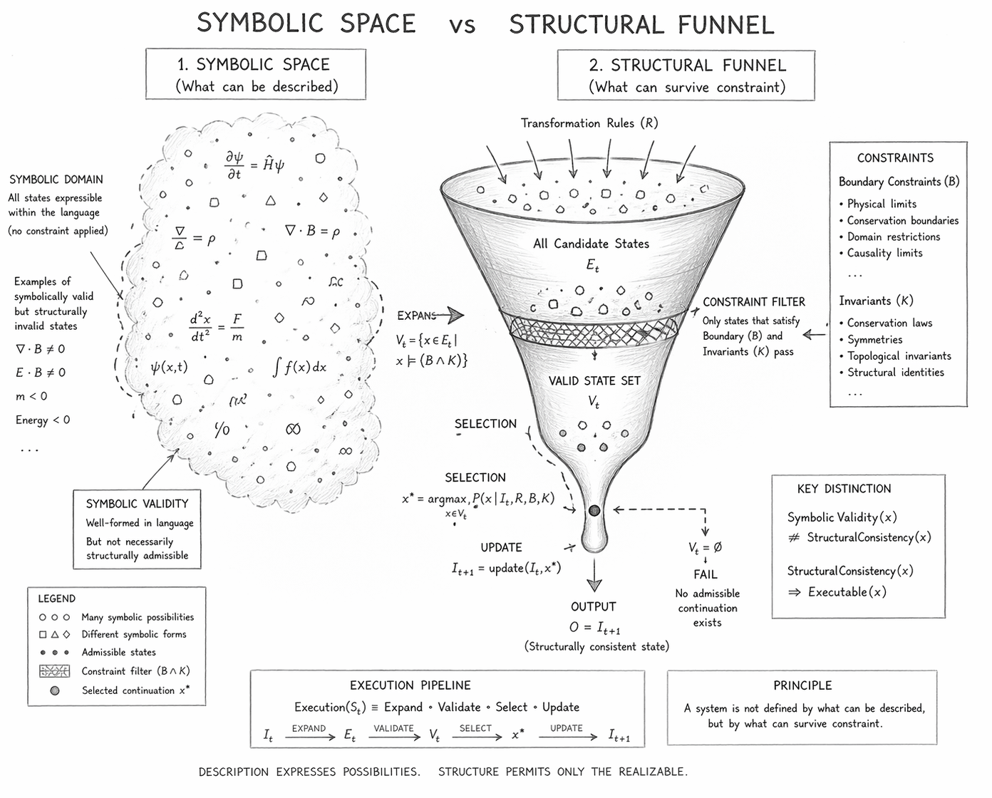
Symbolic Space vs Structural Funnel

1. Overview of the Diagram

This diagram presents a formal distinction between two fundamentally different domains:

  • Symbolic Space — the set of all states that can be expressed within a language
  • Structural Funnel — the subset of states that can survive constraint and execute

The visual structure encodes the transition from unconstrained representability to constraint-governed admissibility, aligning directly with the Flow Algebra execution pipeline.

2. Left Domain: Symbolic Space (Descriptive Superset)

The left-hand region illustrates a diffuse “cloud” of symbolic expressions.

This domain represents:

  • All syntactically valid forms D(x)D(x)
  • All mathematically expressible states
  • All configurations permitted by language rules alone

Key properties:

  • Unbounded expressibility
  • No intrinsic constraint enforcement
  • Coexistence of valid and invalid states

The diagram explicitly includes examples such as:

  • Physically inconsistent equations
  • Violations of conservation laws
  • Ill-defined or non-executable expressions

These illustrate a critical principle:

SymbolicValidity(x)⇏StructuralConsistency(x)

Thus, the symbolic domain is a superset of all possible descriptions, not a guarantee of realizability.

3. Expansion Interface: Transition to Structural Processing

The arrow labeled Expansion represents:

\[ E_t = \operatorname{expand}(I_t, R) \]

This is the bridge between:

  • Static symbolic representation
  • Dynamic generative structure

All candidate states—both valid and invalid—enter the structural system at this stage.

Importantly:

  • No filtering has yet occurred
  • The system remains agnostic to validity at this point

4. Central Structure: The Constraint Funnel

The funnel represents the core mechanism of structural consistency enforcement.

4.1 Upper Funnel — Candidate State Set

The wide opening contains:

\[ E_t \]

This is the full set of generated possibilities:

4.2 Constraint Filter Layer

The narrowing section represents:

\[ x \models (B \land K) \]

This is the critical filtration boundary, enforcing:

  • Boundary Constraints (B)
  • Physical limits
  • Domain restrictions
  • Causality conditions
  • Invariants (K)
  • Conservation laws
  • Symmetries
  • Structural identities

Only states satisfying both are allowed to pass.

This implements:

  • Hard constraint enforcement
  • Immediate rejection of invalid states
  • Elimination without interpretation

5. Lower Funnel: Valid State Set

The reduced set:

\[ V_t \]

represents all structurally admissible states.

Key properties:

  • Constraint-compliant
  • Executable
  • Physically and logically consistent

This is no longer a descriptive space—it is a survival set.


6. Selection Mechanism

Within the valid set, the diagram shows:

\[ x^{*} = \operatorname*{arg\,max}_{x \in V_t} \; P\!\left(x \mid I_t, R, B, K\right) \]

This stage represents:

  • Controlled choice within admissible space
  • Deterministic or probabilistic selection

Critically:

  • Selection does not introduce new states
  • It operates strictly within VtV_t

7. Update and Output

The selected state propagates through:

\[ I_{t+1} = \operatorname{update}(I_t, x^{*}) \]

Producing:

\[ O = I_{t+1} \]

This output is guaranteed to satisfy:

\[ O \models (B \land K) \]

Thus:

  • Every output is structurally valid
  • No invalid state can emerge from the system

8. Failure Condition: Structural Termination

The diagram explicitly includes:

\[ V_t = \emptyset \;\Rightarrow\; \mathrm{FAIL} \]

This represents:

  • Absence of admissible continuation
  • Mandatory system termination

Interpretation:

  • The system refuses to evolve under violation
  • No approximation or symbolic fallback is allowed

Failure is therefore:

  • A consistency-preserving mechanism
  • Not an error, but a logical necessity

9. Right Panel: Constraint Definition Layer

The diagram isolates constraints into two formal categories:

Boundary Constraints (B):
  • External limits
  • Domain-specific restrictions
  • Causal structure
Invariants (K):
  • Conservation laws
  • Symmetries
  • Topological or structural constants

This separation clarifies:

  • What restricts behaviour externally
  • What must remain unchanged internally

10. Key Distinction Block

The diagram highlights the core theoretical result:

SymbolicValidity(x)=StructuralConsistency(x)

StructuralConsistency(x)⇒Executable(x)

This formalises the chapter’s central claim:

Description does not define reality—constraint does.

11. Execution Pipeline (Bottom Strip)

The diagram concludes with the execution identity:

Execution(St​)=Expand→Validate→Select→Update

This provides:

  • A complete operational definition
  • A closed-loop system evolution model

12. Global Interpretation

The diagram encodes a fundamental transformation:

  • From symbolic possibility space
  • To structurally admissible reality

It demonstrates that:

  • Language permits many states
  • Structure permits only a subset
  • Reality corresponds to the subset that survives

Closing Scientific Statement

This diagram is not illustrative—it is operational.

It defines a system in which:

  • All generation is unconstrained initially
  • All continuation is strictly constrained
  • All outputs are guaranteed to preserve invariants

The symbolic domain expresses possibilities.

The structural system determines existence.

What survives constraint is what becomes real.

Diagram → Flow Mapping Table

Diagram Element Flow Algebra Expression Formal Role Scientific Meaning (Ultra-Tight)
Symbolic Space Cloud \( D(x) \) Representation Layer All describable states (no constraint enforcement)
Symbolic Domain Label \( \mathrm{well\_formed}(D(x)) \) Syntax Condition Language-valid expressions
Mixed Valid/Invalid Points \( x \in E_t \) Candidate States Includes both admissible and non-admissible states
Expansion Arrow \( E_t = \mathrm{expand}(I_t, R) \) Generative Step Produces full candidate state space
Funnel Entry (Wide Top) \( E_t \) Candidate Set Unfiltered possibilities
Transformation Label (\( R \)) \( R \) Rule Set Defines allowable transformations
Constraint Filter Mesh \( x \models (B \wedge K) \) Validation Condition Boundary + invariant enforcement
Funnel Narrowing \( E_t \rightarrow V_t \) Filtering Transition Reduction to admissible state set
Valid State Region \( V_t = \{x \in E_t \mid x \models (B \wedge K)\} \) Admissible Set Structurally consistent states
Eliminated States (Blocked) \( x \not\models (B \wedge K) \) Rejection Condition Removed due to constraint violation
Empty Funnel Case \( V_t = \varnothing \) Failure Condition No valid continuation
FAIL Output Arrow \( V_t = \varnothing \Rightarrow O = \mathrm{FAIL} \) Termination Rule Execution halts to preserve consistency
Selection Node \( x^* \in V_t \) Choice Operator Selected admissible continuation
Probabilistic Selection Annotation \( x^* = \arg\max_{x \in V_t} P(x \mid I_t, R, B, K) \) Ranking Mechanism Optimal selection within valid set
Single Output Path \( |V_t| = 1 \Rightarrow x^* \) Deterministic Case Unique continuation
Update Arrow \( I_{t+1} = \mathrm{update}(I_t, x^*) \) State Transition Evolution to next state
Output Node \( O = I_{t+1} \) Result State Structurally consistent output
Constraint Box (\( B \)) \( B \) Boundary Constraints External limits, domain restrictions
Invariant Box (\( K \)) \( K \) Invariants Preserved quantities, symmetries
Execution Pipeline Strip \( \mathrm{Exec}(S_t) = \mathrm{Expand} \circ \mathrm{Validate} \circ \mathrm{Select} \circ \mathrm{Update} \) Process Definition Structured continuation mechanism
Key Distinction Panel \( \mathrm{SymbolicValidity}(x) \nRightarrow \mathrm{StructuralConsistency}(x) \) Core Principle Description ≠ admissibility
Executability Condition \( x \models (B \wedge K) \Rightarrow \mathrm{Executable}(x) \) Validity Guarantee Only constraint-satisfying states can exist
Legend: Many Symbols \( x \in E_t \) Density Indicator Large unconstrained possibility space
Legend: Filtered States \( x \in V_t \) Reduced Set Indicator Surviving admissible states
Legend: Selected Point \( x^* \) Final Choice Actual continuation

Ultra-Tight Execution Strip (Diagram ↔ Flow)

\[ D(x) \;\rightarrow\; E_t = \operatorname{expand}(I_t, R) \;\rightarrow\; V_t = \left\{ x \;\middle|\; x \models (B \land K) \right\} \]

\[ V_t = \emptyset \;\Rightarrow\; \mathrm{FAIL} \;;\; x^{*} \in V_t \;;\; I_{t+1} = \operatorname{update}(I_t, x^{*}) \]

Execution Guarantee Statement

Structural Consistency vs Symbolic Description

Formal Guarantee

For a system defined as:

\[ S = (I, R, B, K) \]

with execution:

\[ E_t = \operatorname{expand}(I_t, R), \quad V_t = \left\{ x \in E_t \;\middle|\; x \models (B \land K) \right\} \]

the following guarantees hold:

1. Admissibility Guarantee

\[ O \neq \mathrm{FAIL} \;\Rightarrow\; O \models (B \land K) \]

Every produced output:

  • Satisfies all boundary constraints
  • Preserves all invariants

No invalid state can be generated.

2. Non-Existence of Invalid Continuation

\[ x \not\models (B \land K) \;\Rightarrow\; x \notin V_t \]

Any state that violates:

  • A boundary constraint
  • An invariant

is excluded prior to selection.

3. Failure Integrity Guarantee

\[ V_t = \emptyset \;\Rightarrow\; O = \mathrm{FAIL} \]

If no admissible state exists:

  • The system halts deterministically
  • No approximation, substitution, or symbolic fallback occurs

Failure preserves structural integrity.

4. Structural Dominance over Symbolic Form

SymbolicValidity(x)⇏StructuralConsistency(x)

StructuralConsistency(x)⇒Executable(x)

Symbolic description:

Does not imply realizability

Structural consistency:

Fully determines executability

5. Selection Safety Guarantee

\[ x^{*} \in V_t \]

All selections:

  • Occur strictly within the admissible set
  • Cannot introduce constraint violations

Probabilistic choice is bounded by structural validity.

6. Deterministic Closure (Given Fixed Inputs)

\[ (I, R, B, K)\ \text{fixed} \;\Rightarrow\; V_t\ \text{fixed} \]

Given identical:

  • State
  • Rules
  • Constraints
  • Invariants

the admissible state space is invariant across executions.

7. No Hidden Structure Guarantee

\[ H = \emptyset \]

The system contains:

  • No implicit assumptions
  • No external corrections
  • No hidden dependencies

All behaviour arises strictly from (I,R,B,K)(I, R, B, K)

8. Execution Integrity Identity

Execution(St​)≡Expand∘Validate∘Select∘Update

Execution is:

  • Fully defined
  • Closed
  • Non-violating

No step permits deviation from constraint satisfaction.

9. Continuation Guarantee

\[ V_t \neq \emptyset \;\Rightarrow\; \exists\, I_{t+1} \;\text{such that}\; I_{t+1} \models (B \land K) \]

If continuation exists:

It is guaranteed to be structurally valid

10. Final Guarantee Statement

This system guarantees that only structurally admissible states can be produced, selected, or propagated.

If a valid continuation exists, it will be found within VtV_t.
If no valid continuation exists, the system halts without producing an invalid result.

Closing Principle

Execution≡Constraint-Preserving Continuation

A system operating under this flow:

  • Cannot violate its invariants
  • Cannot exceed its boundaries
  • Cannot produce an invalid output

It either evolves coherently—

or it does not evolve at all.
Related Chapters
Kireth Research
38 Thorndale Croft, Wetwang, Driffield
East Riding of Yorkshire YO25 9XZ
Telephone: 01377 236594
Designed By