Chapter 46
Phase as Boundary Memory

Within conventional physics, phase is normally treated as a mathematical quantity describing the relative position of a wave within its oscillatory cycle. Whether describing electromagnetic radiation, quantum wavefunctions, acoustics, or classical harmonic motion, phase determines how waves interfere, reinforce, or cancel one another. Although enormously successful, this interpretation generally treats phase as an instantaneous property of oscillation rather than as a persistent structural feature of space itself.

The Holographic Space-Time (HST) framework proposes a broader interpretation. In this chapter, phase is redefined as boundary memory—the accumulated geometric record of previous coherence evolution embedded within recursive boundary structures. Under this view, phase is not simply an angle measured in radians, but a measurable expression of how boundaries preserve and transport historical coherence.

Instead of asking,

HST asks,

This shift transforms phase from a purely temporal coordinate into a recursively accumulated geometric quantity.

Every coherent system evolves through recursive updates.

Rather than existing independently at each instant,

\[ C_t \rightarrow C_{t+1} \]

the current coherence state carries information inherited from previous states.

This accumulated information forms what HST calls boundary memory.

Mathematically,

\[ M_B=\int_{0}^{t} H\!\left(C(\tau)\right)\,d\tau \]

where

Unlike ordinary storage, this memory is not symbolic.

It is geometric.

The boundary itself remembers its own evolution.

Many physical systems preserve phase over remarkably long distances.

Examples include:

Traditional physics explains this through coherence and low environmental noise.

HST instead proposes an additional geometric interpretation.

A stable phase exists because the recursive boundary has maintained its historical memory.

As long as recursive coherence remains intact,

\[ \Gamma_C>\Gamma_{\min} \]

the stored phase history remains recoverable.

Loss of coherence corresponds directly to degradation of boundary memory.

Conventional formulations often describe phase using

\[ \phi=\omega t-kx \]

Although mathematically complete, this equation contains no explicit mechanism explaining why phase remains coherent after long propagation.

Within HST,

phase evolves recursively,

\[ \phi_{t+1}=\phi_t+\Delta\phi(C_t) \]

Each recursive update contributes another layer to the boundary memory.

Thus,

phase becomes the cumulative result of previous coherence transitions rather than merely elapsed time.

The central proposal of this chapter is that coherent boundaries behave analogously to distributed memory media.

Rather than storing bits,

they store curvature relationships.

Boundary memory therefore consists of

The stored information is represented through the coherence density

\[ \rho_C=\rho(\Gamma_C,M_B) \]

Here memory directly modifies coherence density.

Consequently, phase becomes an emergent property of stored geometry.

Interference traditionally occurs because waves possess different phases.

HST reinterprets this phenomenon geometrically.

Two boundaries interfere constructively when their stored histories are compatible.

They interfere destructively when their historical curvature memories disagree.

Constructive interference therefore corresponds to

\[ M_{B_1}\approx M_{B_2} \]

while destructive interference represents increasing memory mismatch,

\[ \left|M_{B_1}-M_{B_2}\right|\rightarrow\max \]

Interference becomes the comparison of recursive boundary histories rather than merely oscillation angles.

Boundary memory naturally explains why coherent systems preserve information during propagation.

Rather than information travelling independently,

the boundary continuously transports its own accumulated structural history.

The propagation sequence becomes

\[ B_t\rightarrow M_B\rightarrow\rho_C\rightarrow\phi\rightarrow I_t \]

Thus information follows coherence.

The wave is simply the observable manifestation of recursive memory transport.

Quantum mechanics places enormous importance on phase differences.

Observable phenomena including

all depend upon phase relationships.

HST suggests that these quantum phases represent the visible manifestation of deeper recursive boundary memories.

The quantum wavefunction therefore encodes not only probability amplitudes but also accumulated coherence history.

The measurable phase reflects how the recursive boundary has evolved.

This chapter naturally extends several earlier developments in the HST framework.

Chapter 46 introduces the missing historical component.

The boundary not only propagates curvature—it remembers previous curvature.

Geometry therefore acquires temporal persistence through recursive coherence.

One of the profound implications of this framework is that space itself becomes capable of retaining structural history.

This does not imply that space stores information like a computer memory.

Instead, recursive coherence continually reshapes boundary geometry so that previous states influence future evolution.

This recursive dependence may be expressed as

\[ M_B(t+1)=M_B(t)+\Delta C_t \]

Memory is therefore generated naturally through recursive structural evolution.

The HST interpretation replaces the traditional concept of phase angle with a richer geometric quantity.

Instead of

the framework proposes

Observable oscillations become readouts of recursive structural history encoded within coherent boundary geometry.

This reinterpretation unifies several previously separate concepts:

Together they form a single geometric description of how boundaries preserve, transport, and reveal information throughout space-time.

Chapter 46 represents an important conceptual advance in the HST framework by proposing that phase is not merely an instantaneous descriptor of oscillatory motion but the observable expression of accumulated boundary memory.

In this interpretation, coherent boundaries continuously integrate their recursive structural evolution, encoding historical information within their curvature and coherence fields.

Observable phase relationships emerge from this stored geometric history, providing a unified explanation for coherence preservation, long-range interference, and information transport.

Rather than treating phase as an isolated mathematical parameter, HST elevates it to a fundamental property of recursive space-time geometry, where every coherent boundary carries the imprint of its own evolution and reveals that history through measurable phase.

The Phase as Boundary Memory flow is a recursive computational model that formalises one of the central concepts introduced by the Holographic Space-Time (HST) framework: phase is not treated as an instantaneous oscillatory quantity, but as the observable expression of accumulated boundary memory.

Rather than describing phase solely by its position within a periodic cycle, this flow interprets phase as a geometric record produced by the continual recursive evolution of coherent boundaries.

The implementation transforms what is traditionally a kinematic parameter into a dynamically accumulated structural quantity. Every recursive update contributes to a growing memory state, and the measurable phase of the system emerges directly from this stored history.

The flow therefore provides a complete execution pathway linking coherence evolution, boundary memory, phase stability, and interference into a single recursive process.

The execution begins by defining the initial boundary configuration:

where:

Unlike conventional wave equations, which often begin with an initial phase angle, the HST flow begins with boundary coherence. This reflects the principle that oscillatory behaviour is not fundamental; rather, it is an observable consequence of an underlying coherent geometric structure.

At this stage the system establishes:

The boundary therefore becomes the substrate upon which all subsequent information is encoded.

The core engine of the flow is the recursive update

Every iteration represents another moment in the evolution of the coherent structure.

Unlike classical simulations that overwrite previous states, the HST implementation preserves the historical contribution of every update. Each recursive step is treated as a permanent modification of the boundary's structural history.

This recursive evolution allows the system to build long-term geometric continuity instead of relying solely on instantaneous state variables.

The defining operation of the chapter is

where:

This equation formalises the principle that every coherence transition contributes to a cumulative geometric memory.

Importantly, the flow does not treat memory as stored digital information. Instead, memory is represented by changes in boundary organisation, curvature relationships, and coherence structure. The accumulated memory therefore exists intrinsically within the evolving geometry itself.

As recursive updates continue, the boundary progressively acquires a richer structural history.

Once the memory has been updated, the flow advances the phase according to

In conventional wave mechanics, phase evolves directly as a function of time and propagation distance. In contrast, this implementation makes the phase increment dependent upon the evolving coherence state.

Phase is therefore no longer an independent variable.

Instead, it becomes a derived quantity that reflects accumulated recursive boundary evolution.

The observable phase measured by an experiment is interpreted as the current readout of the boundary's stored history.

The recursive memory modifies the coherence density through

This stage links three fundamental quantities:

As memory grows, it alters the structural organisation of the boundary. The density therefore reflects not only present coherence but also the historical evolution that produced it.

The flow thereby creates an explicit coupling between geometry and history.

The implementation continuously evaluates

This acts as a structural integrity test.

If coherence falls below the required threshold, the recursive memory can no longer be maintained.

The flow immediately returns

indicating that:

This mechanism models the loss of coherent phase observed experimentally when systems undergo decoherence.

A key feature of the implementation is

Rather than computing phase independently, the flow explicitly reads phase from the accumulated boundary memory.

This operation is the conceptual heart of the chapter.

The measured phase is interpreted as a direct geometric signature of previous recursive evolution.

In this framework, phase becomes analogous to a structural fingerprint left by the history of coherence rather than merely the instantaneous position of a sinusoidal oscillation.

The flow next evaluates two coherent propagation paths:

Their memory difference is computed as

This comparison determines whether the boundaries possess compatible structural histories.

Small memory differences produce

while large differences generate

The interference process therefore becomes a comparison of recursive boundary memories rather than a comparison of abstract phase angles.

This provides a geometric interpretation of interference phenomena without altering their observable predictions.

Information transport follows the sequence

This sequence demonstrates that information does not propagate independently of geometry.

Instead:

Information therefore remains embedded within coherent boundary evolution throughout the propagation process.

The execution loop continues while

Each recursive cycle performs:

The flow therefore implements a continuously self-consistent recursive memory engine.

Every future state inherits information from every previous state, producing long-range structural continuity.

The implementation contains two principal termination mechanisms.

If

the recursive process terminates because coherent boundary organisation can no longer preserve accumulated memory.

If boundary history becomes discontinuous,

the flow returns

This distinguishes complete decoherence from local structural discontinuities that specifically disrupt the recoverability of phase history.

Taken as a whole, this flow implements a recursive geometric model in which phase is generated by the accumulation of boundary memory rather than by elapsed time alone.

It establishes a causal chain beginning with boundary coherence, continuing through recursive structural evolution, and culminating in measurable phase and interference.

Unlike traditional formulations that treat phase as a primary variable, the HST implementation derives phase from the stored history of coherent geometry.

The resulting model integrates coherence, memory, density, phase, and information transport into a unified recursive framework, where every observable phase relationship carries the imprint of the boundary's previous evolution.

The Phase as Boundary Memory flow implements a recursive coherence engine that continuously accumulates geometric history within evolving boundaries and interprets observable phase as the measurable expression of that stored history.

Beginning with boundary coherence, the flow recursively updates structural organisation, integrates boundary memory, recalculates coherence density, derives phase from accumulated history, and predicts interference through comparisons of independent memory states. Stable phase emerges only while coherence remains above a critical threshold, ensuring that recursive structural continuity is preserved.

In this implementation, phase is elevated from a transient oscillatory parameter to a persistent geometric property, providing a unified computational description of coherence preservation, information transport, and interference within the Holographic Space-Time framework.

The Phase as Boundary Memory Flow Algebra implements a recursive computational framework in which phase is interpreted as the accumulated memory of coherent boundary evolution rather than merely the instantaneous position of a periodic oscillation. Within conventional physics, phase is generally expressed as an angular parameter describing the state of a wave relative to its cycle. While this description accurately predicts interference, diffraction, and resonance phenomena, it does not specify a physical mechanism by which coherent systems preserve phase information over extended distances or times.

The Holographic Space-Time (HST) framework proposes that this apparent persistence arises because coherent boundaries continuously retain the geometric consequences of their previous recursive states. In this implementation, every coherence update contributes to a growing structural memory embedded within the boundary itself. Observable phase is therefore not treated as an independent variable but as the measurable manifestation of this accumulated boundary history.

The flow provides a complete recursive execution model linking boundary formation, coherence evolution, memory accumulation, phase generation, information transport, and interference into a single self-consistent computational process.

The flow begins by constructing the initial coherent boundary,

where Bt represents the physical boundary configuration and Ct represents its corresponding coherence state.

Unlike conventional wave equations that initialise systems using amplitude and phase variables, this implementation begins with geometry. Every subsequent quantity—including memory, phase, and interference—is derived from the evolving coherence of this boundary.

This establishes one of the central principles of HST:

Before phase can exist, a coherent boundary capable of preserving structural information must first be established.

The recursive engine advances the system through repeated coherence updates,

Each iteration represents a structural evolution of the boundary rather than a simple progression in time.

Unlike classical numerical integration, where previous states may simply be overwritten, this recursive process permanently contributes to the historical development of the boundary. Every update becomes part of the boundary's geometric record, allowing the system to retain continuity across successive recursive cycles.

This recursive evolution provides the mechanism by which long-range coherence can be maintained despite continuous structural change.

The defining feature of the implementation is the accumulation of boundary memory,

where

This operation transforms transient coherence updates into persistent structural information.

Rather than storing symbolic information or digital states, the flow accumulates modifications in the boundary's geometric organisation. Every recursive adjustment leaves a measurable imprint upon the coherent structure, allowing the boundary to preserve its own evolutionary history.

Memory therefore becomes an intrinsic geometric property rather than an externally stored quantity.

After updating the boundary memory, the flow advances the observable phase,

Here the phase increment depends directly upon the evolving coherence state.

Unlike conventional formulations where phase advances solely according to propagation distance and elapsed time,

\[ \phi=\omega t-kx \]

the HST implementation derives phase from recursive structural evolution.

Phase therefore becomes a secondary quantity generated by accumulated coherence rather than an independent coordinate describing oscillation.

The observable phase of the system is interpreted as the present expression of the boundary's historical development.

The accumulated memory modifies the coherence density through

where

This step establishes an explicit relationship between structural history and present boundary organisation.

As recursive memory increases, it influences the density of coherent organisation within the boundary. Consequently, the current state of the system reflects both its instantaneous coherence and the cumulative effects of all previous recursive updates.

The boundary therefore becomes a continuously evolving geometric archive.

Throughout execution the flow continually evaluates

This coherence threshold determines whether the boundary can continue preserving its accumulated history.

If the stability falls below the minimum allowable level,

the recursive process returns

At this point:

This provides a geometric interpretation of decoherence as the breakdown of boundary memory rather than merely the randomisation of phase.

One of the most important operations within the flow is

Rather than calculating phase independently, the implementation explicitly reads phase from accumulated boundary memory.

This operation represents the conceptual centre of the chapter.

Phase is no longer treated as an abstract angular coordinate.

Instead, it becomes the measurable signature of recursive structural history stored within the boundary.

Every observed phase value therefore contains information regarding the previous evolution of the coherent geometry.

To determine interference behaviour, the flow evaluates the accumulated memories of two propagation paths,

Their structural difference is calculated as

The resulting comparison determines whether the boundaries possess compatible historical evolution.

When the memory difference remains sufficiently small,

destructive interference emerges.

Within this implementation, interference is interpreted as the compatibility—or incompatibility—of recursive boundary histories rather than simply the alignment of oscillatory phases.

Information propagates through the recursive sequence

This execution chain demonstrates that information remains inseparable from coherent geometry.

Boundary evolution produces memory.

Memory determines coherence density.

Density generates observable phase.

Phase governs measurable interference.

Rather than transporting independent signals through empty space, the flow describes information as travelling within the evolving structure of coherent boundaries themselves.

As long as coherence remains above the stability threshold,

the recursive execution loop continues indefinitely.

Each cycle performs:

Every new state inherits information from all preceding states, producing a continuously evolving geometric memory.

This recursive inheritance allows phase coherence to persist naturally throughout propagation.

The implementation recognises two principal failure mechanisms.

If coherence stability falls below the minimum threshold,

recursive memory can no longer be maintained.

The system terminates in a state of decoherence.

If the accumulated structural history becomes discontinuous,

the flow returns

This condition represents the loss of recoverable geometric history even if portions of the boundary remain locally coherent.

The complete implementation provides a recursive geometric description of how coherent boundaries preserve their structural history and how that history becomes observable as measurable phase. Beginning with an initial coherent boundary, the flow recursively updates coherence, accumulates geometric memory, recalculates coherence density, derives phase from stored history, and predicts interference by comparing the memory states of multiple propagation paths.

Rather than treating phase as an isolated mathematical parameter, the implementation integrates it into the broader recursive evolution of boundary geometry. Phase, coherence, memory, density, and information transport become successive manifestations of a single underlying process.

The Phase as Boundary Memory flow implements one of the central theoretical advances of the Holographic Space-Time framework by redefining phase as an emergent property of recursive boundary evolution. Instead of viewing phase as a purely temporal or oscillatory coordinate, the model treats it as a persistent geometric memory encoded within coherent boundary structures.

Through recursive coherence updates, the boundary continuously accumulates structural history, which in turn determines coherence density, generates observable phase, and governs interference behaviour.

This implementation unifies concepts traditionally treated separately—coherence, phase, information storage, propagation, and interference—into a single recursive computational framework, providing a geometric mechanism by which coherent systems preserve and reveal their evolutionary history across space-time.

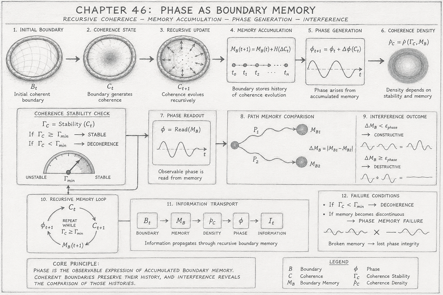
The scientific pencil diagram for Chapter 46 — Phase as Boundary Memory illustrates one of the central concepts of the Holographic Space-Time (HST) framework: phase is not treated as an isolated oscillatory parameter but as the observable expression of recursively accumulated boundary memory.

Rather than depicting phase as an abstract angle advancing through time, the diagram visualises how coherent boundaries continuously record their own structural evolution, allowing observable phase to emerge naturally from accumulated geometric history.

The illustration is organised as a complete recursive execution sequence. Beginning with the formation of a coherent boundary, it follows the successive processes of coherence generation, recursive structural evolution, memory accumulation, phase production, coherence stability monitoring, path comparison, interference generation, and information transport.

Each panel corresponds directly to one stage of the Flow Algebra, providing a visual representation of the mathematical relationships developed throughout the chapter.

The first panel depicts the formation of the initial coherent boundary.

\[ B_t \]

The circular boundary symbol represents the geometric surface from which all later phenomena emerge. Unlike conventional wave diagrams that begin with an oscillating waveform, the HST model begins with the boundary itself, emphasising that geometry is the primary physical object.

The lightly sketched interior indicates that, although the boundary exists, no structural memory has yet accumulated. This represents the initial condition of the recursive system before any history has been encoded.

The second panel shows the boundary developing an organised coherence distribution.

\[ B_t \rightarrow C_t \]

The gradual darkening toward the centre symbolises the emergence of coherent organisation throughout the boundary.

Rather than representing energy concentration, the shading illustrates increasing structural order. At this stage the boundary acquires the capacity to preserve information through recursive evolution, providing the physical foundation from which memory and phase will later emerge.

The third panel illustrates recursive evolution.

\[ C_t \rightarrow C_{t+1} \]

Multiple directional arrows indicate that coherence evolves continuously through self-referential updates. Unlike simple propagation through space, the recursive arrows demonstrate that every new state is generated from the previous coherent configuration.

This panel emphasises that the system possesses internal continuity, where each iteration permanently contributes to the overall structural history.

The fourth panel introduces one of the defining concepts of the chapter.

\[ M_B(t+1)=M_B(t)+H(\Delta C_t) \]

A sequence of discrete memory markers connected by a timeline represents the accumulation of structural history. Each marker corresponds to one recursive update of the coherent boundary. The history operator transforms successive coherence changes into permanently stored geometric information.

Importantly, the illustration avoids depicting digital memory cells or symbolic storage. Instead, the boundary itself becomes the storage medium, with memory encoded directly within its evolving geometric organisation.

The fifth panel depicts the emergence of phase.

\[ \phi_{t+1}=\phi_t+\Delta\phi(C_t) \]

A sinusoidal waveform is drawn not as an independent oscillation but as the observable consequence of accumulated boundary memory. The horizontal progression of the waveform illustrates that phase evolves continuously through recursive coherence updates rather than simply advancing according to elapsed time.

Within the HST interpretation, the wave represents the visible manifestation of deeper geometric history stored within the coherent boundary.

The sixth panel illustrates the relationship

\[ \rho_C=\rho(\Gamma_C,M_B) \]

The increasingly dark circular shading represents the strengthening of coherent density resulting from stable recursive memory. The dense central region symbolises that coherence density depends jointly upon present structural stability and accumulated boundary history.

This visual element reinforces the concept that the current state of the boundary cannot be separated from its previous recursive evolution.

The stability panel introduces the governing threshold

\[ \Gamma_C\geq\Gamma_{\min} \]

The gauge-like indicator represents the health of the recursive boundary. When the pointer remains above the stability threshold, recursive memory continues to accumulate. If the pointer falls below the threshold, the boundary loses its ability to preserve structural history.

This panel represents the control mechanism that determines whether phase remains recoverable or whether decoherence occurs.

The next panel introduces the defining operation of the chapter:

\[ \phi=\operatorname{Read}(M_B) \]

The waveform beneath the equation illustrates that observable phase is extracted directly from accumulated boundary memory. Rather than computing phase independently, the recursive system measures the current state of its stored geometric history.

This panel provides perhaps the most important conceptual transition in the entire diagram. Phase is no longer fundamental; it becomes a measurable consequence of recursive structural evolution.

The diagram then divides into two independent propagation paths.

\[ P_1,\;P_2 \]

Each path accumulates its own boundary memory,

\[ M_{B_1},\;M_{B_2} \]

The comparison

\[ \Delta M_B=\left|M_{B_1}-M_{B_2}\right| \]

determines the compatibility of their structural histories.

Unlike conventional interference diagrams that compare wave crests and troughs directly, this illustration compares the historical evolution of two coherent boundaries. The interference pattern therefore reflects the agreement—or disagreement—between recursive memories rather than instantaneous oscillation angles.

The interference panel presents two possible outcomes.

For compatible memories,

\[ \Delta M_B<\varepsilon_{\mathrm{phase}} \]

constructive interference occurs.

For incompatible memories,

\[ \Delta M_B\geq\varepsilon_{\mathrm{phase}} \]

destructive interference results.

The paired waveforms illustrate that observable interference is interpreted as the geometric comparison of accumulated boundary histories. The visual transition from reinforcement to cancellation symbolises how differences in recursive memory determine measurable interference behaviour.

The circular loop illustrates the continuous recursive execution engine.$$C_t \rightarrow C_{t+1} \rightarrow M_B(t+1) \rightarrow \phi_{t+1} \rightarrow C_t$$

\[ C_t\rightarrow C_{t+1}\rightarrow M_B(t+1)\rightarrow \phi_{t+1}\rightarrow C_t \]

Unlike a linear computational pipeline, this closed cycle demonstrates that every newly generated phase contributes to future recursive evolution. The system therefore continuously updates its own boundary memory while simultaneously generating new observable phase relationships.

This panel highlights one of the defining characteristics of HST: recursive self-consistency.

The information transport chain summarises the complete execution sequence:

\[ B_t\rightarrow M_B\rightarrow\rho_C\rightarrow\phi\rightarrow I_t \]

Each block represents one stage of the recursive transformation.

Boundary geometry generates memory.

Memory modifies coherence density.

Coherence density produces observable phase.

Observable phase carries measurable information.

The diagram therefore demonstrates that information remains inseparable from coherent geometric evolution throughout the entire propagation process.

The final panel illustrates the two principal failure mechanisms.

The first occurs when

\[ \Gamma_C<\Gamma_{\min} \]

causing complete decoherence.

The second occurs when accumulated boundary memory becomes discontinuous, producing Phase Memory Failure.

The broken waveform symbolises the inability of the boundary to reconstruct a continuous phase history once recursive structural continuity has been lost.

At the bottom of the diagram, the boxed summary encapsulates the chapter's principal scientific statement:

This statement unifies every component of the diagram into a single geometric interpretation. Rather than existing as an isolated wave parameter, phase emerges as the measurable signature of recursive coherence preserved within evolving boundary geometry.

Viewed as a whole, the diagram presents a complete recursive execution model for the HST interpretation of phase. Beginning with the formation of a coherent boundary, it shows how recursive coherence updates accumulate structural memory, how that memory determines coherence density, how observable phase is extracted from stored history, and how interference arises through the comparison of independent boundary memories.

Every panel builds upon the previous one, forming a continuous causal chain that replaces the conventional interpretation of phase as an instantaneous oscillatory coordinate with a geometric description based on recursive memory.

The illustration therefore serves as both a visual summary of the chapter and a direct graphical representation of the accompanying Flow Algebra, demonstrating that phase, memory, coherence, information, and interference are successive manifestations of a single recursive boundary process within the Holographic Space-Time framework.

The diagram provides a one-to-one visual mapping of the Flow Algebra for Phase as Boundary Memory. Every graphical element corresponds directly to a mathematical operation and a stage of recursive execution.

The progression begins with the formation of a coherent boundary, advances through recursive coherence updates and boundary memory accumulation, generates observable phase from stored geometric history, compares the memories of independent propagation paths to determine interference, and concludes by either preserving recursive evolution or terminating when coherence is lost.

The complete mapping illustrates the central HST proposition that phase is the observable readout of accumulated boundary memory, making coherence, memory, information transport, and interference successive expressions of a single recursive geometric process.

The Phase as Boundary Memory Flow Algebra is a deterministic recursive execution model that guarantees a unique computational outcome for every valid boundary state satisfying the coherence constraints defined by the Holographic Space-Time (HST) framework.

Beginning with an initial coherent boundary, the flow recursively updates the coherence field, accumulates boundary memory, derives observable phase from stored structural history, evaluates coherence stability, compares independent memory states, and produces a measurable interference output. Every stage possesses explicitly defined inputs, outputs, transition rules, and termination conditions, ensuring that the execution path is fully specified and reproducible.

Unlike conventional procedural algorithms that treat phase as an externally supplied parameter, this flow guarantees that phase is generated internally as the deterministic consequence of recursive boundary evolution. No stage requires arbitrary parameter insertion or undefined intermediate states once the initial boundary configuration has been established.

Execution always begins from the initial boundary

\[ B_t \]

which produces the initial coherence state

\[ B_t\rightarrow C_t \]

The recursive update

\[ C_t\rightarrow C_{t+1} \]

is deterministic.

For an identical boundary configuration and identical recursive update operator, the resulting coherence evolution will always be identical.

No probabilistic branching occurs within the flow.

Boundary memory evolves according to

\[ M_B(t+1)=M_B(t)+H(\Delta C_t) \]

For every recursive coherence update there exists exactly one corresponding memory increment generated by the history operator.

Therefore,

The recursive history remains uniquely defined throughout execution.

Observable phase is computed using

\[ \phi_{t+1}=\phi_t+\Delta\phi(C_t) \]

followed by

\[ \phi=\operatorname{Read}(M_B) \]

Since boundary memory is uniquely determined, the resulting phase is likewise uniquely determined.

The flow therefore guarantees that phase cannot evolve independently of recursive structural history.

Every observable phase corresponds to one and only one accumulated boundary memory state.

Throughout execution the stability condition

\[ \Gamma_C\geq\Gamma_{\min} \]

is continuously evaluated.

If the condition remains true,

the recursive execution proceeds without interruption.

If

\[ \Gamma_C<\Gamma_{\min} \]

execution immediately enters the predefined DECOHERENCE state.

No undefined intermediate condition exists.

Every execution therefore terminates in either:

The flow guarantees the preservation of causal ordering through the execution sequence

\[ B_t\rightarrow M_B\rightarrow\rho_C\rightarrow\phi\rightarrow I_t \]

Each quantity depends only upon previously computed quantities.

No future state is required to calculate a previous state.

Consequently:

For two coherent propagation paths,

\[ M_{B_1},\;M_{B_2} \]

the comparison

\[ \Delta M_B=\left|M_{B_1}-M_{B_2}\right| \]

always produces one unique interference classification.

If

\[ \Delta M_B<\varepsilon_{\mathrm{phase}} \]

the execution returns

Constructive Interference.

Otherwise,

\[ \Delta M_B\geq\varepsilon_{\mathrm{phase}} \]

returns

Destructive Interference.

No ambiguous interference state exists.

Every execution cycle satisfies

\[ (C_t,M_B,\phi_t)\rightarrow(C_{t+1},M_B(t+1),\phi_{t+1}) \]

Each recursive update preserves structural continuity by ensuring that:

No recursive state can be skipped, repeated, or reordered.

Execution terminates only under explicitly defined conditions.

If

\[ \Gamma_C\geq\Gamma_{\min} \]

the recursive memory engine continues indefinitely while preserving coherent phase.

If

\[ \Gamma_C<\Gamma_{\min} \]

execution terminates with

If accumulated boundary memory becomes discontinuous,

\[ \neg\operatorname{Continuous}(M_B) \]

execution terminates with

These termination criteria completely define the allowable execution space.

The flow guarantees that every valid execution performs the complete sequence

\[ B_t\rightarrow C_t\rightarrow C_{t+1}\rightarrow M_B\rightarrow\rho_C\rightarrow\phi\rightarrow I_t \]

No stage may be omitted.

No additional hidden operations are required.

The execution therefore remains computationally complete.

Throughout execution the following invariants remain preserved:

\[ B_t\neq\varnothing \]

A valid boundary always exists.

\[ M_B(t+1)=M_B(t)+H(\Delta C_t) \]

Memory is accumulated without loss while coherence remains stable.

\[ \Gamma_C\geq\Gamma_{\min} \]

Stable coherence guarantees recoverable boundary memory.

\[ \phi=\operatorname{Read}(M_B) \]

Observable phase is always derived from accumulated structural history.

\[ B_t\rightarrow M_B\rightarrow\rho_C\rightarrow\phi\rightarrow I_t \]

Information always propagates through the same deterministic execution pathway.