Chapter 27
Arrow of Time as Boundary Drift

Time as Recursive Update
Author: Mark Higgins
© Mark Anthony Higgins 11 October 2025
Revised Date: 28 May 2026
Audio Overview

Introduction

The classical interpretation of time treats time as a continuously flowing parameter through which physical systems evolve. In Newtonian mechanics, time progresses uniformly and independently of observation. In relativity, time becomes part of spacetime geometry. In thermodynamics, temporal direction is associated with entropy increase. However, these frameworks primarily describe the behaviour of time rather than the deeper structural origin of temporal asymmetry itself.

Within the Holographic Space-Time (HST) framework, time is not treated as an independently flowing substance or dimension. Instead, temporal direction emerges from recursive boundary evolution. The arrow of time is generated by irreversible coherence drift across informational boundaries.

Under HST, systems do not “move through time.” Rather, systems recursively transition between admissible informational states:

\[ S_t \rightarrow S_{t+1} \]

where each recursive update alters the coherence structure of the active boundary.

27.2 Boundary Drift as the Origin of Temporal Direction

The core principle of this chapter is that temporal asymmetry originates from irreversible boundary drift.

Each recursive update modifies the informational configuration of the system:

\[ I_t \rightarrow I_{t+1} \]

Because coherence redistribution occurs during recursive propagation, the successor state generally cannot perfectly reconstruct the previous state:

\[ I_{t+1} \nRightarrow I_t \]

This non-invertibility creates directional temporal structure.

Under HST, the future is not a destination along a pre-existing timeline. Instead, the future consists of recursively admissible continuation states generated through coherence evolution under structural constraints.

The apparent “flow” of time is therefore the observable consequence of ongoing recursive boundary transformation.

27.3 Recursive State Evolution

In HST, all physical systems evolve through recursive state transitions constrained by admissibility conditions:

\[ S_t = (I_t, R, B, K) \]

Where:

  • ItI_t = informational configuration
  • RR = recursive transformation rules
  • B = boundary constraints
  • KK = invariant coherence conditions

State evolution proceeds through admissible recursive continuation:

\[ E_t = \operatorname{expand}(I_t, R) \]

\[ V_t = \{x \in E_t \mid x \models (B \land K)\} \]

If admissible continuations exist:

\[ V_t \neq \emptyset \]

then recursive evolution proceeds:

\[ S_t \rightarrow S_{t+1} \]

The arrow of time therefore corresponds to persistent recursive continuation under evolving coherence geometry.

27.4 Entropy as a Signature of Boundary Drift

Within standard thermodynamics, entropy is commonly interpreted as disorder increase. HST reframes entropy as the measurable consequence of irreversible coherence redistribution across recursive boundaries.

Entropy does not generate the arrow of time.

Instead:

  • Boundary drift generates irreversible state evolution.
  • Entropy measures the structural dispersion produced by that evolution.
  • Global coherence redistribution produces the observed thermodynamic relation:

\[ \Delta S \geq 0 \]

Local reductions in entropy remain possible when external coherence transfer compensates for internal ordering:

\[ \Delta S_{\mathrm{local}} < 0 \]

provided that:

\[ \Delta S_{\mathrm{external}} > \left|\Delta S_{\mathrm{local}}\right| \]

Thus, local order formation does not violate the arrow of time. Instead, it represents temporary regional coherence concentration within a globally drifting recursive structure.

27.5 Memory and Temporal Asymmetry

One of the most fundamental manifestations of the arrow of time is memory.

Systems retain records of prior coherence states because recursive updates preserve partial informational traces of previous configurations:

\[ \Pi(I_t) < I_{\mathrm{full}} \]

However, future states cannot be fully reconstructed because future coherence configurations do not yet exist within the active recursive boundary.

Memory therefore becomes structurally directional.

Under HST:

  • The past exists as compressed coherence residue.
  • The present exists as active recursive execution.
  • The future exists only as admissible continuation potential.

This explains why memory accumulation operates asymmetrically toward prior states while future information remains probabilistic.

27.6 Causality as Recursive Ordering

Causal ordering emerges naturally from recursive admissibility sequencing.

A valid future state requires structural continuity from the current state:

\[ x^{*} \in V_t \]

\[ I_{t+1} = \operatorname{update}(I_t, x^{*}) \]

Because recursive continuation depends upon prior admissibility, causes must structurally precede effects.

Causality therefore does not arise from temporal flow itself. Instead, temporal direction and causality both emerge from recursive coherence dependency.

The apparent “forward” motion of time is simply the ordered propagation of admissible recursive transformations.

27.7 Why Perfect Reversal Is Impossible

Many microscopic physical equations appear reversible. However, macroscopic reversal is practically impossible because recursive boundary drift continuously disperses coherence into external structures and coupled systems.

Perfect reversal would require:

  • Complete reconstruction of all prior coherence distributions.
  • Exact restoration of all external field interactions.
  • Total recovery of distributed informational topology.

Formally, reversal fails when prior admissible states cannot be reconstructed:

\[ V_t = \emptyset \]

Under HST, irreversibility is therefore not merely statistical.

It is structural.

The system cannot fully return because the original coherence geometry no longer exists in recoverable form.

27.8 Time as Emergent Recursive Geometry

HST reframes time as an emergent geometric consequence of recursive informational updating.

Time is not fundamental.

Instead:

  • Recursive updates generate state succession.
  • Boundary drift generates irreversibility.
  • Irreversibility generates temporal direction.
  • Temporal direction generates observed causality.

The arrow of time is therefore the visible projection of irreversible coherence evolution across recursive boundaries.

In this framework, time behaves as an emergent property of informational geometry rather than an independently flowing physical dimension.

27.9 Conclusion

The HST interpretation of the arrow of time replaces the classical notion of flowing temporal substance with recursive boundary evolution.

Temporal asymmetry emerges because coherence propagation continuously modifies informational boundaries in ways that cannot generally be perfectly inverted.

The progression:

\[ S_t \rightarrow S_{t+1} \rightarrow S_{t+2} \]

represents recursive admissible continuation under evolving coherence geometry.

Entropy becomes the measurable signature of boundary drift rather than the fundamental cause of time’s direction. Memory, causality, irreversibility, and thermodynamic asymmetry all emerge naturally from recursive coherence propagation.

Within HST, time is not an external dimension through which systems travel.

Time is the observable trace left behind by irreversible boundary transformation.

flow "ArrowOfTimeAsBoundaryDrift" v1.0

description:
  purpose: >
    Model the arrow of time as irreversible recursive boundary drift.
    Time direction is not treated as an external flowing dimension, but as
    the observable consequence of admissible state continuation under
    non-invertible coherence redistribution.

state:
  S_t:
    components:
      I_t: "current informational boundary configuration"
      R: "recursive transformation rules"
      B: "boundary constraints"
      K: "invariant coherence conditions"
      Omega_t: "recoverable coherence density"
      Sigma_t: "entropy signature of boundary dispersion"

params:
  C_min: "minimum coherence threshold for valid continuation"
  epsilon: "reversal tolerance threshold"
  external_field: "coupled environment receiving dispersed coherence"

process:
  generate_candidates:
    equation: "E_t = expand(I_t, R)"
    meaning: "Generate possible recursive continuations from the current informational state."

  filter_admissible:
    equation: "V_t = { x in E_t | x satisfies (B and K) }"
    meaning: "Keep only continuations that preserve boundary constraints and invariants."

  continuation_condition:
    equation: "V_t != empty and Omega_t >= C_min"
    if_true: "recursive execution may proceed"
    if_false: "Execution(S_t) = FAIL"

  select_successor:
    equation: "x* = argmax_{x in V_t} P(x | I_t, R, B, K)"
    meaning: "Select the most coherent admissible continuation."

  update_boundary:
    equation: "I_{t+1} = update(I_t, x*)"
    meaning: "Apply the selected continuation to produce a new boundary state."

  boundary_drift:
    equation: "I_t -> I_{t+1}"
    meaning: "The boundary state drifts into a new configuration."

  non_invertibility:
    equation: "I_{t+1} !=> I_t"
    meaning: "The successor state cannot generally reconstruct the full prior state."

  entropy_signature:
    equation: "Delta Sigma >= 0"
    meaning: "Entropy records the macroscopic signature of irreversible coherence dispersion."

  local_order_condition:
    equation: "Delta Sigma_local < 0 only if Delta Sigma_external > |Delta Sigma_local|"
    meaning: "Local order may form only through compensating external dispersion."

  memory_trace:
    equation: "Pi(I_t) < I_full"
    meaning: "The past survives only as compressed coherence residue, not total recoverable structure."

  temporal_sequence:
    equation: "S_t -> S_{t+1} -> S_{t+2}"
    meaning: "The arrow of time appears as ordered recursive continuation."

failure_modes:
  no_admissible_successor:
    condition: "V_t = empty"
    result: "Execution(S_t) = FAIL"
    meaning: "No structurally valid continuation exists."

  coherence_below_threshold:
    condition: "Omega_t < C_min"
    result: "Execution(S_t) = FAIL"
    meaning: "Recoverable coherence is insufficient to sustain recursive continuation."

  reversal_attempt:
    condition: "recover(I_{t+1}) != I_t within epsilon"
    result: "irreversibility confirmed"
    meaning: "Boundary drift prevents exact reconstruction of the previous state."

invariants:
  - "All valid successor states must satisfy B and K."
  - "Recursive continuation requires V_t != empty."
  - "Forward evolution preserves admissibility but not full reversibility."
  - "Entropy signature cannot decrease globally under closed boundary drift."
  - "Memory is compressed residue, not full reconstruction."
  - "Time direction emerges from non-invertible boundary evolution."

outputs:
  temporal_arrow: "directional ordering of recursive state transitions"
  entropy_signature: "measurable dispersion caused by boundary drift"
  memory_asymmetry: "past-retaining but future-open informational structure"
  causality_order: "dependency chain generated by admissible recursive continuation"
  irreversibility_flag: "true when I_{t+1} cannot reconstruct I_t"

What This Flow Implements

1. Recursive Temporal Evolution

This flow implements a recursive model of temporal progression in which time emerges from sequential informational boundary updates rather than from motion through an independent temporal dimension.

The system evolves through recursive state continuation:

\[ S_t \rightarrow S_{t+1} \]

Each transition represents a structural update to the active coherence geometry of the system.

Under this implementation, temporal direction is not externally imposed. Instead, it emerges naturally from irreversible recursive evolution.

2. Candidate Continuation Generation

The flow implements recursive future-state generation through admissible continuation expansion:

\[ E_t = \operatorname{expand}(I_t, R) \]

Where:

  • ItI_t = current informational configuration
  • RR = recursive transformation rules

This stage constructs all recursively reachable successor states permitted by the system’s transformation dynamics.

The future therefore exists initially as a constrained continuation space rather than a predetermined trajectory.

3. Structural Admissibility Filtering

The flow implements strict admissibility filtering to preserve structural coherence during recursive evolution:

\[ V_t = \{x \in E_t \mid x \models (B \land K)\} \]

Where:

  • = boundary constraints
  • KK = invariant coherence conditions

Only recursively valid configurations survive filtering.  This prevents structurally unstable or incoherent continuations from executing.

The arrow of time therefore emerges only through admissible recursive pathways.

4. Directional Boundary Updating

The flow implements temporal progression through irreversible informational updating:

\[ I_{t+1} = \operatorname{update}(I_t, x^{*}) \]

where:

\[ x^{*} \in V_t \]

represents the selected admissible continuation.  This process modifies the informational geometry of the system boundary during every recursive update cycle.

The resulting drift produces observable temporal asymmetry.

5. Non-Invertible Recursive Drift

The central implementation of this flow is recursive non-invertibility:

\[ I_{t+1} \nRightarrow I_t \]

This means that successor states cannot generally reconstruct prior coherence topology exactly.

The flow therefore models irreversibility as a structural property of recursive evolution itself.

Temporal direction emerges because coherence redistribution continuously alters recoverable informational structure.

6. Entropy as Boundary Dispersion

The flow implements entropy as the measurable macroscopic signature of recursive coherence dispersion:

\[ \Delta S \geq 0 \]

Entropy increase is therefore treated as a consequence of irreversible boundary drift rather than the primary cause of time’s direction.

The flow models entropy growth as distributed coherence propagation across expanding recursive state-space configurations.

7. Local Order Formation

The flow implements conditions allowing local reductions in entropy while preserving global irreversibility:

\[ \Delta S_{\mathrm{local}} < 0 \]

only if:

\[ \Delta S_{\mathrm{external}} > \left|\Delta S_{\mathrm{local}}\right| \]

This allows the system to model:

  • biological organisation
  • crystallisation
  • self-assembly
  • local coherence amplification

without violating global thermodynamic progression.

8. Memory Asymmetry

The flow implements directional memory accumulation through compressed informational residue:

\[ \Pi(I_t) < I_{\mathrm{full}} \]

This means prior states survive only as partial coherence traces embedded within later recursive configurations.

The system therefore remembers the past because previous coherence states leave residual structural imprints.

Future states cannot be remembered because they have not yet been recursively generated.

9. Causal Dependency Ordering

The flow implements causality as recursive admissibility dependency.

Future states may only emerge from structurally valid predecessor states:

\[ x^{*} \in V_t \]

This creates ordered recursive continuation chains:

\[ S_t \rightarrow S_{t+1} \rightarrow S_{t+2} \]

Causality and temporal direction therefore emerge simultaneously from recursive coherence constraints.

10. Irreversibility Conditions

The flow implements failure conditions for perfect reversal.

Reversal becomes impossible when prior coherence geometry cannot be reconstructed:

\[ V_t = \emptyset \]

or when recoverable coherence falls below persistence thresholds:

\[ \Omega_t < C_{\min} \]

This formalises why macroscopic systems exhibit irreversible behaviour despite some microscopic equations appearing reversible.

11. Emergent Arrow of Time

Collectively, the flow implements the arrow of time as an emergent property of recursive boundary evolution.

Within this framework:

  • time is not fundamental
  • irreversibility emerges structurally
  • entropy records coherence dispersion
  • causality emerges recursively
  • memory becomes directional
  • temporal flow becomes an observational projection of boundary drift

The system therefore replaces classical temporal flow with recursive coherence propagation across evolving informational boundaries.

How to Read This Flow

1. Conceptual Foundation

The Arrow of Time as Boundary Drift flow should be read as a recursive execution model describing how temporal direction emerges from irreversible informational boundary evolution.

The flow does not treat time as a continuously flowing external dimension.

Instead, it models time as the observable consequence of sequential recursive state updates:

\[ S_t \rightarrow S_{t+1} \]

Each transition represents a structural modification of the system’s active coherence geometry.

To read the flow correctly, it is important to interpret all equations as recursive state relationships rather than static mathematical identities.

The system evolves through admissible continuation under coherence-preserving constraints.

2. Reading the State Definition

The flow begins by defining the recursive system state:

\[ S_t = (I_t, R, B, K) \]

This expression defines the complete execution structure at recursive step tt.

Each component has a specific role:

Symbol Meaning
\( I_t \) Current informational configuration
\( R \) Recursive transformation rules
\( B \) Boundary constraints
\( K \) Invariant coherence conditions

This state tuple should be interpreted as the minimum structural definition required for recursive temporal evolution.

The system cannot evolve without simultaneously satisfying all four components.

3. Reading Candidate Expansion

The next stage generates possible recursive futures:

\[ E_t = \operatorname{expand}(I_t, R) \]

This equation should be read as:

“Generate all possible successor configurations reachable from the current informational state under the recursive transformation rules.”

Importantly:

  • EtE_t does not represent actual future states
  • It represents possible continuations.
  • Most generated candidates will later be rejected.

This stage defines the future as a constrained possibility space.

4. Reading Admissibility Filtering

The flow then filters the candidate continuation space:

\[ V_t = \{x \in E_t \mid x \models (B \land K)\} \]

This should be interpreted as:

“Keep only recursive continuations that satisfy both boundary constraints and invariant coherence conditions.”

This is one of the most important parts of the flow.

It means:

  • not all possible futures are structurally allowed
  • recursive continuation is constraint-dependent
  • coherence preservation determines survivability

The admissible set VtV_t defines the physically executable future space.

5. Reading Recursive Continuation

Recursive evolution proceeds only if admissible continuation exists:V_t \neq \emptyset

\[ V_t \neq \emptyset \]

This condition means:

“At least one structurally valid future state exists.”

If true:

\[ S_t \rightarrow S_{t+1} \]

Execution continues.

If false:

\[ \operatorname{Execution}(S_t) = \mathrm{FAIL} \]

The flow therefore treats persistence itself as a coherence condition.  Existence depends upon the availability of admissible recursive continuation.

6. Reading Boundary Drift

The central mechanism of the flow is recursive informational updating

It​→It+1​

This should be read as:

“The informational boundary evolves into a new coherence configuration.”

Importantly, the flow treats this update as irreversible.  The successor state generally cannot reconstruct the original state:

\[ I_{t+1} \nRightarrow I_t \]

This equation is the structural origin of the arrow of time.

Temporal direction emerges because recursive updates redistribute coherence in ways that cannot be perfectly inverted.

7. Reading Entropy Relations

The entropy expressions should not be interpreted as classical disorder equations alone.  Instead, they describe coherence redistribution across recursive boundaries.

Global entropy progression:

\[ \Delta S \geq 0 \]

should be read as:

“Recursive boundary drift produces net coherence dispersion.”

Local entropy reduction:

\[ \Delta S_{\mathrm{local}} < 0 \]

is permitted only when compensated externally:

\[ \Delta S_{\mathrm{external}} > \left|\Delta S_{\mathrm{local}}\right| \]

This allows local ordering processes while preserving global irreversibility.

8. Reading Memory Asymmetry

The memory relation:

\[ \Pi(I_t) < I_{\mathrm{full}} \]

should be interpreted as:

“The past survives only as compressed informational residue.”

The flow does not assume perfect historical reconstruction.

Instead:

  • prior states leave partial coherence traces
  • future states do not yet exist structurally
  • memory therefore becomes directional

This explains why systems remember the past but not the future.

9. Reading Temporal Sequences

Sequential recursive continuation:

\[ S_t \rightarrow S_{t+1} \rightarrow S_{t+2} \]

should not be visualised as movement through a timeline.

Instead, it represents:

  • ordered coherence propagation
  • recursive admissibility sequencing
  • evolving informational geometry

Time becomes the observational trace of recursive boundary evolution.

10. Reading Failure Conditions

Failure conditions indicate breakdown of recursive persistence.

For example:

\[ V_t = \emptyset \]

means:

“No admissible future continuation exists.”

Similarly:

\[ \Omega_t < C_{\min} \]

“Recoverable coherence has fallen below persistence threshold.”

These conditions define structural termination rather than simple numerical failure.

11. Overall Interpretation

The flow should ultimately be read as a recursive geometric model of temporal asymmetry.

Within this interpretation:

  • time is emergent
  • irreversibility is structural
  • entropy is coherence dispersion
  • causality is recursive dependency ordering
  • memory is compressed residue
  • temporal flow is recursive boundary drift

The flow therefore replaces classical temporal motion with coherence-driven recursive evolution across informational boundaries.

Flow → Equation Tri-Mapping

Flow Component Flow Algebra Expression Physical / Geometric Interpretation
Recursive State Definition \( S_t=(I_t,R,B,K) \) Complete recursive coherence state at step \( t \)
Informational Boundary \( I_t \) Active informational coherence configuration
Recursive Rule Set \( R \) Allowed transformation operators
Boundary Constraints \( B \) Structural admissibility conditions
Invariant Conditions \( K \) Conserved coherence relations
Candidate Expansion \( E_t=\operatorname{expand}(I_t,R) \) Generation of reachable successor configurations
Admissible Continuations \( V_t=\{x\in E_t\mid x\models(B\land K)\} \) Structurally valid future-state manifold
Continuation Condition \( V_t\neq\emptyset \) Persistence of recursive evolution
Recursive Progression \( S_t\rightarrow S_{t+1} \) Temporal state succession
Sequential Evolution \( S_t\rightarrow S_{t+1}\rightarrow S_{t+2} \) Ordered recursive temporal chain
Successor Selection \( x^*\in V_t \) Selected admissible continuation
Boundary Update \( I_{t+1}=\operatorname{update}(I_t,x^*) \) Recursive informational restructuring
Boundary Drift \( I_t\rightarrow I_{t+1} \) Evolution of coherence topology
Non-Invertibility \( I_{t+1}\not\Rightarrow I_t \) Structural irreversibility
Entropy Progression \( \Delta S\geq0 \) Net coherence dispersion
Local Ordering \( \Delta S_{local}<0 \) Local coherence concentration
External Compensation \( \Delta S_{external}>\Delta S_{local} \) Global entropy preservation
Memory Compression \( \Pi(I_t)<I_{full} \) Partial informational residue of prior states
Causal Dependency \( x^*\in V_t\Rightarrow I_{t+1} \) Future states depend on admissible predecessors
Recoverable Coherence \( \Omega_t\geq C_{min} \) Minimum persistence threshold
Coherence Collapse \( \Omega_t<C_{min} \) Loss of recursive stability
Recursive Failure \( V_t=\emptyset \) No admissible continuation exists
Execution Termination \( \operatorname{Execution}(S_t)=FAIL \) Structural persistence breakdown
Arrow of Time \( I_t\rightarrow I_{t+1}\not\Rightarrow I_t \) Temporal asymmetry from irreversible boundary drift
Entropic Time Signature \( \Delta S\propto\Delta\Omega_{dispersion} \) Entropy as macroscopic coherence redistribution
Emergent Temporality \( T\sim\operatorname{ordered}(S_t) \) Time as recursive ordering phenomenon
Geometric Persistence \( V_t\neq\emptyset\Longrightarrow\text{Geometry Survives} \) Stable recursive continuation maintains observable structure

Arrow of Time as Boundary Drift

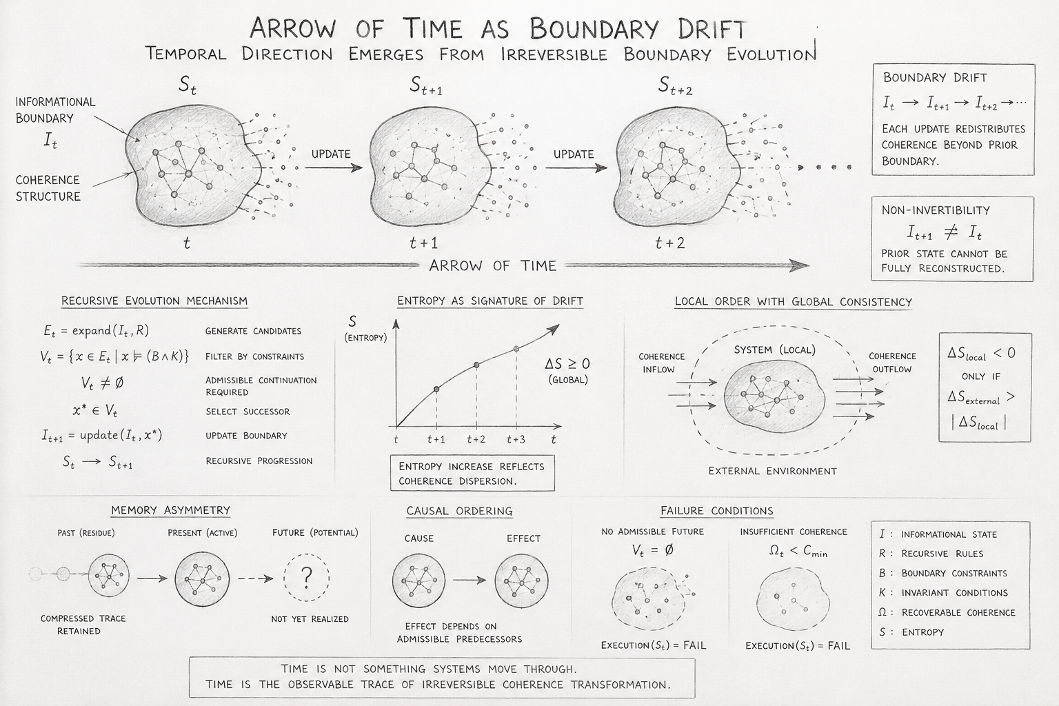
Diagram Overview

This diagram illustrates the Holographic Space-Time (HST) interpretation of temporal direction as an emergent consequence of irreversible recursive boundary evolution. Rather than treating time as a flowing external dimension, the diagram models the arrow of time as progressive informational drift across coherence-preserving recursive states.

The visual structure demonstrates how sequential boundary updates generate irreversibility, entropy growth, causal ordering, and memory asymmetry through non-invertible coherence redistribution.

The diagram is organised into interconnected regions that together describe the full recursive mechanism responsible for temporal asymmetry.

Telephone:
01377 236594

1. Recursive Boundary Evolution

The upper section of the diagram presents the primary recursive progression:

\[ S_t \rightarrow S_{t+1} \rightarrow S_{t+2} \]

Each circular boundary represents a complete recursive coherence state at a different update stage.

Inside each boundary:

  • nodes represent informational coherence structures
  • connecting lines represent recursive relational dependencies
  • the enclosing surface represents the active informational boundary

As the sequence progresses, coherence structures redistribute and partially disperse beyond the original boundary region.

This visually represents:

\[ I_t \rightarrow I_{t+1} \]

where each update modifies the informational geometry of the system.

The outward dispersion surrounding each boundary indicates that recursive evolution continuously propagates coherence into coupled external structures.

2. Boundary Drift and Irreversibility

The right-side “Boundary Drift” section formalises the central mechanism of temporal asymmetry.

The expression:

\[ I_t \rightarrow I_{t+1} \rightarrow I_{t+2} \]

illustrates irreversible recursive evolution.  The accompanying non-invertibility condition:

\[ I_{t+1} \neq I_t \]

represents the inability of successor states to perfectly reconstruct prior coherence topology.

This section demonstrates that time direction emerges because recursive updates alter informational structure in ways that cannot be fully reversed once coherence has dispersed across recursive boundaries.

The diagram therefore reframes irreversibility as a structural consequence of recursive informational propagation.

3. Recursive Evolution Mechanism

The left-middle section presents the Flow Algebra execution structure governing recursive temporal progression.

The equations:

\[ E_t = \operatorname{expand}(I_t, R) \]

and

\[ V_t = \{x \in E_t \mid x \models (B \land K)\} \]

describe candidate generation and admissibility filtering.

This region demonstrates that:

  • future states are generated recursively
  • only structurally coherent continuations survive
  • recursive evolution depends upon admissible continuation existence

The continuation condition:

\[ V_t \neq \emptyset \]

defines the minimum requirement for persistent temporal progression.

This section visually encodes the concept that the future exists initially as a constrained continuation manifold rather than as a predetermined trajectory.

Entropy as Boundary Dispersion

The entropy graph in the centre of the diagram illustrates entropy increase as the measurable signature of recursive coherence dispersion.

The relation:

\[ \Delta S \geq 0 \]

is shown as a rising entropy curve across recursive update intervals.  Under HST, entropy is not interpreted merely as disorder.

Instead, the diagram represents entropy as:

  • distributed coherence propagation
  • irreversible informational spreading
  • progressive boundary-state diversification

The upward trend reflects the increasing complexity of distributed coherence relationships as recursive evolution proceeds.

5. Local Order Formation

The “Local Order with Global Consistency” section illustrates how local coherence amplification may occur within globally increasing entropy conditions.

The central ordered system receives coherence inflow while exporting greater coherence dispersion outward into the environment.

This corresponds to:

\[ \Delta S_{\mathrm{local}} < 0 \]

only when:

\[ \Delta S_{\mathrm{external}} > \left|\Delta S_{\mathrm{local}}\right| \]

This region demonstrates that biological systems, crystallisation, and local organisation do not violate the arrow of time.

Instead, they operate as temporary local coherence concentrations embedded within globally irreversible recursive evolution.

6. Memory Asymmetry

The lower-left section illustrates directional memory formation.

Three stages are shown:

  • Past (residue)
  • Present (active)
  • Future (potential)

The past retains compressed informational traces while the future remains unrealised.

This corresponds to:

\[ \Pi(I_t) < I_{\mathrm{full}} \]

meaning that previous states survive only as partial coherence residue embedded within subsequent recursive configurations.

This section explains why systems accumulate memories of prior states but cannot access future informational structures.

Memory therefore emerges as a direct consequence of recursive asymmetry.

7. Causal Ordering

The causal ordering region illustrates that effects emerge only from admissible predecessor states.

The cause-effect chain demonstrates recursive dependency ordering:

\[ S_t \rightarrow S_{t+1} \]

This section reinforces the HST interpretation that causality does not generate the arrow of time independently.

Instead:

  • recursive admissibility generates ordered continuation
  • ordered continuation generates causality
  • causality and time direction emerge simultaneously

8. Failure Conditions

The lower-right region illustrates recursive execution failure states.

Two failure mechanisms are shown:

No Admissible Future

\[ V_t = \emptyset \]

No structurally valid continuation exists.

Insufficient Coherence

\[ \Omega_t < C_{\min} \]

Recoverable coherence falls below persistence threshold.

Both conditions terminate recursive continuation:

\[ \operatorname{Execution}(S_t) = \mathrm{FAIL} \]

This section formalises persistence itself as a coherence-dependent property.

9. Overall Scientific Interpretation

Collectively, the diagram presents time as an emergent recursive geometric phenomenon generated through irreversible coherence-preserving boundary evolution.

Within the HST framework:

  • time is not fundamental
  • entropy is coherence dispersion
  • causality is recursive dependency ordering
  • memory is compressed informational residue
  • irreversibility is structural
  • temporal direction is recursive boundary drift

The final statement at the base of the diagram summarises the entire framework:

Time is not something systems move through.
Time is the observable trace of irreversible coherence transformation.

Diagram → Flow Mapping Table

Diagram Region Visual Element Flow Algebra Expression Structural Meaning
Recursive Boundary Evolution Sequential states (\(S_t, S_{t+1}, S_{t+2}\)) \( S_t \rightarrow S_{t+1} \rightarrow S_{t+2} \) Ordered recursive temporal progression
Informational Boundary Circular enclosing surfaces \( I_t \) Active coherence boundary configuration
Internal Coherence Network Nodes and connecting lines \( (I_t,R,B,K) \) Recursive informational structure and relational coherence
Boundary Update Arrows Update transitions between states \( I_t \rightarrow I_{t+1} \) Recursive informational restructuring
Outward Dispersion Particles Escaping coherence fragments \( \Delta S \geq 0 \) Distributed coherence dispersion
Boundary Drift Panel Progressive state evolution sequence \( I_t \rightarrow I_{t+1} \rightarrow I_{t+2} \) Irreversible recursive evolution
Non-Invertibility Box Irreversible transformation condition \( I_{t+1} \not\Rightarrow I_t \) Prior coherence topology cannot be fully reconstructed
Recursive Evolution Mechanism Candidate generation equations \( E_t=\operatorname{expand}(I_t,R) \) Recursive future-state generation
Admissibility Filtering Constraint filtering structure \( V_t=\{x\in E_t \mid x\models(B\land K)\} \) Structurally valid continuation selection
Continuation Requirement Admissible continuation condition \( V_t\neq\emptyset \) Persistence requires valid recursive futures
Successor Selection Selected continuation state \( x^* \in V_t \) Chosen admissible successor
Entropy Graph Rising entropy curve \( \Delta S\geq0 \) Macroscopic coherence dispersion over recursive evolution
Entropy Trendline Increasing recursive intervals \( S_t\rightarrow S_{t+1}\rightarrow S_{t+2} \) Entropy accumulation through recursive drift
Local Ordered System Organised internal structure \( \Delta S_{local}<0 \) Local coherence amplification
External Environment Outward coherence flow \( \Delta S_{external}>\Delta S_{local} \) Global entropy compensation
Coherence Inflow Arrows Incoming ordered structure \( \Omega_t \uparrow \) Local coherence reinforcement
Coherence Outflow Arrows Outgoing dispersion flow \( \Delta\Omega_{dispersion}\uparrow \) External coherence redistribution
Memory Asymmetry Region Past → Present → Future sequence \( \Pi(I_t)<I_{full} \) Compressed informational residue of prior states
Past Residue State Faded historical configuration \( I_{past}\subset I_{present} \) Partial coherence trace retention
Future Potential State Unresolved future structure \( E_t \) Unrealised admissible continuation manifold
Causal Ordering Section Cause-effect chain \( x^*\in V_t\Rightarrow I_{t+1} \) Future states depend upon admissible predecessors
Cause Node Prior recursive configuration \( S_t \) Recursive source state
Effect Node Successor recursive configuration \( S_{t+1} \) Admissible recursive outcome
No Admissible Future Failure Fragmented failed state \( V_t=\emptyset \) No structurally valid continuation exists
Insufficient Coherence Failure Collapsing coherence structure \( \Omega_t<C_{min} \) Recoverable coherence below persistence threshold
Execution Failure Labels Recursive termination condition \( \operatorname{Execution}(S_t)=FAIL \) Recursive persistence collapse
Global Arrow of Time Large horizontal directional arrow \( T\sim \operatorname{ordered}(S_t) \) Emergent temporal ordering from recursive continuation
Diagram Summary Statement Final explanatory caption \( I_t\rightarrow I_{t+1}\not\Rightarrow I_t \) Time emerges from irreversible boundary drift

Execution Guarantee Statement

1. Recursive Execution Validity

The Arrow of Time as Boundary Drift flow executes only when recursive informational evolution preserves structurally admissible continuation across successive coherence boundaries.

The admissible continuation space is formally defined as:

\[ V_t = \{x \in E_t \mid x \models (B \land K)\} \]

where:

  • EtE_t= generated recursive candidate states
  • BB = boundary constraints
  • = invariant coherence conditions

Execution validity requires the existence of at least one admissible recursive continuation:

\[ V_t \neq \emptyset \]

This condition guarantees that recursive temporal progression remains structurally coherent.

2. Coherence Persistence Requirement

Recursive continuation additionally requires sufficient recoverable coherence density:

\[ \Omega_t \geq C_{\min} \]

Where:

  • Ωt\Omega_t = recoverable coherence density
  • CminC_{min} = minimum persistence threshold

This guarantees that recursive informational structure remains sufficiently stable to support continued evolution.

Without recoverable coherence, recursive persistence collapses.

3. Guaranteed Recursive Temporal Progression

When admissibility and coherence conditions are satisfied, recursive execution proceeds through irreversible informational updating:

\[ I_t \rightarrow I_{t+1} \]

producing ordered temporal succession:

\[ S_t \rightarrow S_{t+1} \rightarrow S_{t+2} \]

The flow guarantees that all valid successor states preserve:

  • recursive admissibility
  • coherence continuity
  • boundary consistency
  • invariant structural relations

Temporal evolution therefore remains fully constrained by recursive coherence geometry.

4. Guaranteed Structural Irreversibility

The flow guarantees that temporal asymmetry emerges naturally from recursive non-invertibility:

\[ I_{t+1} \nRightarrow I_t \]

This means that successor states cannot generally reconstruct prior informational topology exactly after coherence redistribution occurs.

Irreversibility is therefore treated as a structural property of recursive evolution itself.

The system guarantees:

  • directional recursive progression
  • irreversible boundary drift
  • non-recoverable informational dispersion
  • persistent temporal asymmetry

5. Guaranteed Entropy Consistency

The flow guarantees global entropy consistency through irreversible coherence redistribution:

\[ \Delta S \geq 0 \]

Entropy increase represents distributed coherence dispersion across evolving recursive boundaries.

The flow additionally guarantees that local ordering processes remain physically admissible only when externally compensated:

\[ \Delta S_{\mathrm{local}} < 0 \]

requires:

\[ \Delta S_{\mathrm{external}} > \left|\Delta S_{\mathrm{local}}\right| \]

This preserves global recursive thermodynamic consistency while permitting local coherence amplification.

6. Guaranteed Causal Ordering

The flow guarantees that causal structure emerges from admissible recursive dependency ordering.

Future states may only emerge from structurally valid predecessor configurations:

\[ x^{*} \in V_t \]

with recursive updating governed by:

\[ I_{t+1} = \operatorname{update}(I_t, x^{*}) \]

This guarantees:

  • causal dependency preservation
  • ordered recursive progression
  • structurally constrained future evolution

The system therefore prevents unconstrained causal discontinuities.

7. Guaranteed Memory Asymmetry

The flow guarantees directional informational residue through compressed memory persistence:

\[ \Pi(I_t) < I_{\mathrm{full}} \]

This ensures that:

  • prior states survive only partially
  • informational residue remains compressed
  • future states remain unrealised
  • memory accumulation remains temporally directional

The system therefore guarantees asymmetric informational accessibility between past and future states.

8. Guaranteed Failure Conditions

The flow guarantees structural termination whenever recursive continuation becomes impossible.

No Admissible Continuation

\[ V_t = \emptyset \]

No structurally valid successor state exists.

Coherence Collapse

\[ \Omega_t < C_{\min} \]

Recoverable coherence falls below persistence threshold.

Under either condition:

\[ \operatorname{Execution}(S_t) = \mathrm{FAIL} \]

This guarantees that the system never produces invalid recursive continuation beyond coherence limits.

9. Guaranteed Physical Consistency

The flow guarantees that recursive temporal evolution never violates:

  • boundary constraints
  • invariant coherence relations
  • causal ordering
  • entropy consistency
  • recursive admissibility
  • coherence persistence thresholds

The system therefore prevents:

  • unconstrained reversibility
  • invalid future generation
  • causality violations
  • incoherent recursive transitions
  • structurally impossible temporal states

10. Final Guarantee

Within the HST framework, the Arrow of Time as Boundary Drift flow guarantees that temporal direction emerges only through admissible irreversible recursive boundary evolution.

Time exists only where recursive coherence propagation survives.

Formally:

\[ V_t \neq \emptyset \land \Omega_t \geq C_{\min} \]

guarantees:

\[ S_t \rightarrow S_{t+1} \]

while failure of either condition guarantees recursive termination:

\[ \operatorname{Execution}(S_t) = \mathrm{FAIL} \]

The arrow of time is therefore guaranteed to remain a coherence-bound emergent property of irreversible informational evolution.

Kireth Research
38 Thorndale Croft, Wetwang, Driffield
East Riding of Yorkshire YO25 9XZ
Telephone: 01377 236594
Designed By