Chapter 21
Coherence Gradients

PART II — Coherence Geometry
Author: Mark Higgins
© Mark Anthony Higgins 11 October 2025
Revised Date: 18 May 2026
Audio Overview

21.1 Introduction

Modern physics describes many natural phenomena through gradients.
Temperature gradients drive thermodynamics. Pressure gradients drive fluid motion. Potential gradients generate electromagnetic acceleration. Curvature gradients shape gravitational dynamics.

In each case, motion emerges not from isolated objects acting independently, but from differential structure distributed across a field.

Holographic Space-Time (HST) extends this principle further by proposing that coherence itself possesses measurable gradient structure.

Within HST, coherence is not treated as an abstract philosophical property or informational metaphor. Instead, coherence is defined as the degree of recursive structural compatibility maintained across interacting boundary-encoded systems. Differences in coherence density generate directional structural tension, producing organized flow, curvature migration, phase alignment, and energy redistribution.

A coherence gradient therefore represents a spatial or relational variation in recursive admissibility.

Rather than interpreting dynamics purely through force exchange, HST reformulates many physical processes as systems seeking locally stable coherence configurations under invariant-preserving constraints.

21.2 Definition of a Coherence Gradient

A coherence gradient is defined as:

A directional variation in structural admissibility density across a recursive field configuration.

Formally:

\[ \nabla C \neq 0 \]

where:

CC represents local coherence density,

∇C\nabla C represents the coherence gradient field.

Regions with higher coherence possess greater recursive stability, admissibility preservation, and invariant compatibility.

Regions with lower coherence contain elevated contradiction density, instability, fragmentation pressure, or unresolved boundary tension.

The resulting gradient produces directional system evolution toward recursively sustainable states.

In HST:

\[ \mathrm{Flow\ Direction} \propto \nabla C \]

meaning that systems naturally evolve along coherence differentials.

21.3 Coherence as Structural Potential

Classical physics often uses potential fields:

  • gravitational potential,
  • electric potential,
  • chemical potential,
  • pressure potential.

HST generalizes this idea into structural potential.  A coherence field represents the recursive survivability landscape of admissible configurations.

Systems embedded within such a landscape tend to move toward:

  • reduced contradiction,
  • improved recursive closure,
  • invariant preservation,
  • lower structural tension.

Thus coherence gradients function similarly to generalized stability potentials.

The critical distinction is that HST does not define motion primarily through force particles or external pushes, but through recursive admissibility optimization across boundary geometries.

21.4 Gradient-Driven Structural Motion

Within HST, motion emerges when local coherence imbalance exists.

If two regions possess unequal coherence density:

\[ C_A \neq C_B \]

then recursive pressure develops across the boundary.

This produces:

  • curvature redistribution,
  • information flow,
  • energy transfer,
  • geometric migration,
  • synchronization behavior,
  • phase correction.

The stronger the coherence differential:

\[ \left| \nabla C \right| \]

the stronger the induced structural flow tendency.  This framework unifies numerous phenomena under a single structural principle.

Examples include:

Physical Phenomenon HST Interpretation
Heat flow Coherence equalization
Diffusion Recursive density smoothing
Gravity Curvature coherence descent
Electromagnetic attraction Boundary phase alignment
Quantum collapse Local coherence stabilization
Biological organization Multi-scale coherence optimization

21.5 Coherence Gradients and Geometry

In HST, geometry is not primary.

Geometry emerges from recursive informational organization:

\[ D = G(I) \]

where geometry DD is generated from informational structure II.

Coherence gradients therefore modify geometry indirectly by altering recursive admissibility structure.

This leads to:

  • curvature formation,
  • geometric compression,
  • topological stabilization,
  • boundary deformation,
  • spacetime flow behavior.

Under this interpretation, spacetime curvature itself becomes a secondary manifestation of deeper coherence differentials.

Gravity can therefore be reinterpreted as:

Recursive motion along coherence descent pathways within boundary-encoded geometric structure.
Telephone:
01377 236594

21.6 Local vs Global Coherence Fields

HST distinguishes between:

Local Coherence

Short-range recursive stabilization within confined systems.

Examples:

  • atomic orbitals,
  • molecular bonds,
  • biological cells,
  • local electromagnetic structures.
Global Coherence

Large-scale recursive alignment across extended systems.

Examples:

  • planetary fields,
  • galactic structure,
  • cosmological curvature balance,
  • distributed biological ecosystems.

Coherence gradients may exist simultaneously across multiple scales:

\[ \nabla C_{\mathrm{local}} \quad \text{and} \quad \nabla C_{\mathrm{global}} \]

with cross-scale interactions producing emergent phenomena.

This multi-scale coherence structure becomes essential for understanding complex systems.

21.7 Gradient Collapse and Instability

If coherence gradients become excessively steep, recursive instability may occur.

This produces:

  • contradiction amplification,
  • boundary rupture,
  • phase decoherence,
  • energetic discharge,
  • collapse transitions.

Formally

\[ \left| \nabla C \right| \rightarrow \infty \;\Rightarrow\; \mathrm{Recursive\ Instability} \]

Examples include:

  • lightning discharge,
  • phase transitions,
  • turbulence,
  • quantum decoherence,
  • catastrophic structural collapse.

Stable systems therefore require bounded coherence gradients.

21.8 Recursive Equilibrium

Equilibrium occurs when coherence gradients sufficiently minimize:

\[ \nabla C \approx 0 \]

This does not imply static inactivity.

Instead, equilibrium represents dynamically sustained recursive balance.  A stable coherent system may continue evolving internally while preserving invariant compatibility globally.

Thus equilibrium in HST is not stillness, but sustainable recursive continuity.

21.9 Coherence Gradients as a Universal Structural Principle

The HST framework proposes that coherence gradients form a universal organizing mechanism underlying:

  • physical motion,
  • energetic redistribution,
  • information flow,
  • biological self-organization,
  • cognitive stabilization,
  • social synchronization,
  • cosmological evolution.

Rather than treating these as isolated domains, HST interprets them as manifestations of the same recursive structural law operating at different scales.

This establishes coherence gradients as one of the foundational dynamical engines of recursive reality.

21.10 Chapter Summary

This chapter introduced coherence gradients as directional variations in recursive structural admissibility.

Key principles established include:

  • coherence behaves as a measurable structural field,
  • gradients produce directional system evolution,
  • geometry emerges secondarily from coherence structure,
  • motion reflects recursive admissibility optimization,
  • equilibrium corresponds to sustained recursive balance,
  • instability emerges from excessive coherence differential.

Within HST, coherence gradients provide a unified structural mechanism connecting thermodynamics, gravity, quantum behavior, biological organization, and large-scale cosmological evolution into a single recursively admissible framework.

flow "CoherenceGradients" v1.0

# ---------------------------------------------------------
# PURPOSE
# ---------------------------------------------------------

purpose:
  Define coherence gradients as recursive structural
  differentials that generate directional admissible flow,
  curvature redistribution, and stability-seeking evolution
  across recursive systems.

# ---------------------------------------------------------
# CORE STATE
# ---------------------------------------------------------

state:
  S_t = (I_t, R, B, K)

where:

  I_t:
    Current recursive informational configuration.

  R:
    Recursive transformation operators governing
    admissible structural evolution.

  B:
    Boundary admissibility constraints defining
    allowable recursive continuation.

  K:
    Structural invariants preserved during evolution.

# ---------------------------------------------------------
# COHERENCE FIELD
# ---------------------------------------------------------

coherence_field:

  C(x,t):
    Local coherence density at position x and time t.

definition:
  CoherenceDensity ≡ RecursiveAdmissibilityDensity

properties:
  - local_stability
  - recursive_alignment
  - invariant_compatibility
  - contradiction_minimization
  - boundary_consistency

# ---------------------------------------------------------
# COHERENCE GRADIENT
# ---------------------------------------------------------

gradient:

  ∇C = spatial_gradient(C)

definition:
  CoherenceGradient ≡ DirectionalVariationOfRecursiveAdmissibility

conditions:

  if ∇C = 0:
    state = recursive_equilibrium

  if ∇C ≠ 0:
    state = directed_structural_flow

# ---------------------------------------------------------
# RECURSIVE EXPANSION
# ---------------------------------------------------------

expansion:

  E_t = expand(I_t,R)

definition:
  Generates all reachable recursive continuations.

# ---------------------------------------------------------
# ADMISSIBILITY FILTER
# ---------------------------------------------------------

validation:

  V_t = {x ∈ E_t | x ⊨ (B ∧ K)}

definition:
  Filters all candidate states according to
  recursive admissibility and invariant preservation.

# ---------------------------------------------------------
# FLOW DIRECTION
# ---------------------------------------------------------

flow_dynamics:

  F_c ∝ ∇C

definition:
  Structural flow emerges along coherence differentials.

effects:
  - curvature_shift
  - energy_redistribution
  - phase_alignment
  - geometric_reconfiguration
  - recursive_stabilization

# ---------------------------------------------------------
# STRUCTURAL MOTION
# ---------------------------------------------------------

motion:

  if C_A ≠ C_B:
    recursive_pressure = true

result:
  system_evolves_toward:
    - lower_contradiction
    - higher_admissibility
    - invariant_preservation
    - recursive_stability

# ---------------------------------------------------------
# GEOMETRIC EMERGENCE
# ---------------------------------------------------------

geometry:

  D = G(I)

definition:
  Geometry emerges from recursive informational structure.

constraint:
  D ⇏ (I,R,B,K)

meaning:
  Geometry cannot generate or repair recursion independently.

# ---------------------------------------------------------
# STABILITY CONDITION
# ---------------------------------------------------------

stability:

  Stable(S_t) ⟺ ∀t, I_t ⊨ (B ∧ K)

meaning:
  Stability exists only when recursive continuation
  preserves admissibility and invariants.

# ---------------------------------------------------------
# INSTABILITY CONDITION
# ---------------------------------------------------------

instability:

  if |∇C| → ∞:
    RecursiveInstability = true

effects:
  - decoherence
  - contradiction_amplification
  - boundary_rupture
  - energetic_discharge
  - collapse_transition

# ---------------------------------------------------------
# EQUILIBRIUM
# ---------------------------------------------------------

equilibrium:

  ∇C ≈ 0

meaning:
  Dynamic recursive balance exists across the system.

note:
  Equilibrium does not imply static inactivity.

# ---------------------------------------------------------
# EXECUTION PATH
# ---------------------------------------------------------

execution:

  I_t
    → E_t
    → V_t
    → x*
    → I_t+1

selection:

  x* = argmax_{x∈V_t} P(x | I_t,R,B,K)

meaning:
  The system selects the highest admissible recursive continuation.

# ---------------------------------------------------------
# FAILURE CONDITION
# ---------------------------------------------------------

failure:

  if V_t = ∅:
    Execution = FAIL

meaning:
  No recursively admissible continuation exists.

# ---------------------------------------------------------
# UNIVERSAL INTERPRETATION
# ---------------------------------------------------------

mapping:

  gravity:
    coherence_descent

  thermodynamics:
    coherence_equalization

  electromagnetism:
    phase_alignment_flow

  biology:
    multi_scale_coherence_optimization

  cognition:
    recursive_stabilization_dynamics

  cosmology:
    global_coherence_redistribution

# ---------------------------------------------------------
# EXECUTION GUARANTEE
# ---------------------------------------------------------

guarantee:

  Existence ⟺ V_t ≠ ∅

  RecursiveFlow ⟺ ∇C admissibly propagates through V_t

  Stability ⟺ coherence evolution preserves (B ∧ K)

# ---------------------------------------------------------
# TERMINAL PRINCIPLE
# ---------------------------------------------------------

terminal:

  Recursive systems evolve along admissible
  coherence gradients toward structurally stable states.

What This Flow Implements

Overview

The Coherence Gradients Flow implements a recursive structural model describing how systems evolve through variations in coherence density across admissible informational fields.

Rather than treating motion, organization, or stabilization as isolated force interactions, this flow formalizes the principle that recursive systems naturally evolve along gradients of structural admissibility.

The flow defines coherence as a measurable recursive property governing:

  • stability,
  • continuation,
  • invariant preservation,
  • contradiction minimization,
  • geometric organization.

It then establishes how differences in coherence density generate directional recursive flow across a system.

Core Structural Implementation

1. Recursive System State Definition

The flow begins by constructing the full recursive state:

\[ S_t = (I_t, R, B, K) \]

where:

  • ItI_t represents the active informational configuration,
  • RR defines recursive transformation operators,
  • defines admissibility boundaries,
  • KK defines preserved structural invariants.

This creates the foundational executable recursive substrate upon which coherence dynamics operate.

The flow therefore implements:

Recursive structural state-space evolution under invariant-preserving boundary constraints.

2. Coherence Density Formalization

The flow defines local coherence density:

\[ C(x,t) \]

as the measurable degree of recursive admissibility within a region of the system.

This implementation converts coherence from an abstract philosophical concept into a formal structural field variable.

The flow explicitly models coherence as:

  • local recursive stability,
  • boundary consistency,
  • contradiction minimization,
  • invariant compatibility,
  • recursive survivability.

This enables coherence to become mathematically propagatable across recursive systems.

3. Coherence Gradient Generation

The flow implements the coherence gradient operator:

\[ \nabla C \]

which measures directional variation in recursive admissibility density.  This is one of the central mechanisms of the chapter.

The implementation establishes that:

  • regions of unequal coherence produce recursive pressure,
  • recursive pressure induces directional evolution,
  • systems naturally propagate toward higher admissibility states.

Thus the flow operationalizes:

\[ F_c \propto \nabla C \]

where structural flow emerges directly from coherence differentials.

4. Recursive Expansion and Candidate Generation

The flow implements recursive expansion:

\[ E_t = \operatorname{expand}(I_t, R) \]

This generates all reachable recursive continuations available from the current state. Importantly, the system does not immediately select arbitrary outcomes.

Instead, all possible recursive continuations are first structurally explored.

This creates the admissible continuation space.

5. Admissibility Filtering

The flow then implements recursive validation:

\[ V_t = \left\{ x \in E_t \mid x \models (B \land K) \right\} \]

This stage removes all structurally invalid continuations.

The implementation guarantees that only states satisfying:

  • boundary legality,
  • recursive consistency,
  • invariant preservation

may continue evolving.

This is one of the defining features separating Flow Algebra from unconstrained probabilistic generation systems.

The flow therefore implements:

Constraint-propagated recursive continuation rather than unrestricted generation.

6. Structural Motion and Recursive Pressure

The flow implements directional recursive evolution when coherence imbalance exists:

\[ C_A \neq C_B \]

This produces recursive pressure between regions.

The system then evolves toward:

  • reduced contradiction,
  • increased recursive admissibility,
  • improved structural consistency,
  • stabilized invariant preservation.
This formalizes motion itself as:
Recursive stabilization dynamics across coherence differentials.

7. Geometric Emergence

The flow implements the HST geometric emergence relation:

\[ D = G(I) \]

This states that geometry is generated from recursive informational structure.

The flow additionally enforces:

\[ D \nRightarrow (I, R, B, K) \]

meaning geometry cannot independently generate or repair recursive structure.

This implementation prevents geometric primacy and preserves the foundational role of recursive informational admissibility.

8. Stability and Equilibrium Conditions

The flow implements recursive stability as:

\[ \mathrm{Stable}(S_t) \;\Longleftrightarrow\; \forall t,\; I_t \models (B \land K) \]

A system is stable only when recursive evolution continuously preserves admissibility and invariants.

The flow also defines recursive equilibrium:

\[ \nabla C \approx 0 \]

This does not imply inactivity.

Instead, equilibrium represents dynamically sustained recursive balance.

Thus the implementation supports:

  • active stability,
  • continuous recursive motion,
  • bounded coherence propagation,
  • long-term invariant preservation.

9. Instability and Collapse Dynamics

The flow implements recursive instability conditions:

\[ \left| \nabla C \right| \rightarrow \infty \]

When coherence differentials become excessively steep, recursive stability collapses.

The implementation models:

  • decoherence,
  • contradiction amplification,
  • energetic discharge,
  • boundary rupture,
  • collapse transitions.

This allows the framework to represent both stable and unstable recursive systems under a unified structural mechanism.

10. Recursive Selection and Continuation

The flow implements admissible recursive selection:

\[ x^\ast = \arg\max_{x \in V_t} P(x \mid I_t, R, B, K) \]

Selection occurs only after admissibility filtering.

This guarantees:

  • structurally illegal states cannot be selected,
  • recursive continuation remains invariant-safe,
  • evolution remains boundary-consistent.

The resulting execution path becomes:

\[ I_t \rightarrow E_t \rightarrow V_t \rightarrow x^\ast \rightarrow I_{t+1} \]

11. Failure Detection

The flow explicitly implements recursive failure conditions:

\[ V_t = \emptyset \;\Rightarrow\; \mathrm{Execution} = \mathrm{FAIL} \]

This means:

  • no admissible continuation exists,
  • recursive propagation terminates,
  • contradiction density exceeds survivable structure.

Failure is therefore not arbitrary.

It is structurally defined through the absence of recursively admissible continuation.

12. Universal Physical Interpretation

The flow implements a unified recursive interpretation across multiple domains.

Examples include:

Domain Structural Interpretation
Gravity Coherence descent
Thermodynamics Coherence equalization
Electromagnetism Phase alignment flow
Biology Multi-scale coherence optimization
Cognition Recursive stabilization
Cosmology Global coherence redistribution

This establishes the flow as a universal recursive dynamical framework rather than a domain-specific model.

Final Structural Implementation Statement

The Coherence Gradients Flow implements a fully recursive, boundary-constrained dynamical system in which:

  • coherence behaves as a measurable structural field,
  • gradients generate directional recursive motion,
  • admissibility governs continuation,
  • geometry emerges from recursive information,
  • equilibrium represents sustainable recursive balance,
  • instability emerges from excessive coherence differential,
  • existence itself depends on admissible continuation.

The result is a generalized structural engine capable of describing recursive evolution across physical, informational, biological, cognitive, and cosmological systems within a unified HST-compatible framework.

How to Read This Flow

Overview

The Coherence Gradients Flow describes how recursive systems evolve through directional variations in structural admissibility.

The flow should not be interpreted as conventional software code or symbolic mathematical notation alone.

Instead, it represents:

  • a recursive execution structure,
  • a constraint-preserving evolution system,
  • a coherence propagation model,
  • and a structural description of admissible system dynamics.

The flow is read sequentially from top to bottom, where each section defines a deeper layer of recursive organization.

Importantly:

The flow does not simulate arbitrary motion.

It instead models how systems evolve only through recursively admissible continuations.

1. Read the Flow as a Recursive State Machine

The flow begins with the recursive state definition:

\[ S_t = (I_t, R, B, K) \]

This defines the complete recursive system at time tt.

Read each component as follows:

Component Meaning
\( I_t \) Current informational structure
\( R \) Recursive transformation rules
\( B \) Boundary admissibility constraints
\( K \) Structural invariants

This state is the foundational recursive substrate from which all coherence behavior emerges.

Everything that follows operates upon this recursive state configuration.

2. Interpret Coherence as Structural Admissibility

The flow defines:

\[ C(x,t) \]

as local coherence density.

Do not interpret coherence emotionally or metaphorically.

Within the flow:

Coherence means recursive structural compatibility.

High coherence indicates:

  • low contradiction density,
  • strong invariant compatibility,
  • stable recursive continuation,
  • preserved admissibility.

Low coherence indicates:

  • instability,
  • recursive tension,
  • contradiction accumulation,
  • weakened continuation survivability.

Thus coherence behaves as a measurable recursive field property.

3. Read the Gradient Operator as Directional Structural Difference

The next major operation is:

\[ \nabla C \]

This represents the coherence gradient.

Read this as:

The directional rate of change in recursive admissibility density.

If:

\[ \nabla C = 0 \]

the system is in recursive equilibrium.

If:

\[ \nabla C \neq 0 \]

directional structural flow emerges.

The gradient therefore acts as the primary driver of recursive motion throughout the flow.

4. Read Expansion as Candidate Continuation Generation

The flow next defines:

\[ E_t = \operatorname{expand}(I_t, R) \]

This operation generates all possible recursive continuations reachable from the current state.

Importantly:

  • expansion does not imply validity,
  • generated candidates may still violate constraints,
  • the expansion phase only constructs possibility space.

Thus EtE_t represents:

The total recursive continuation landscape prior to admissibility filtering.

5. Read Validation as Structural Filtering

The flow then defines:

\[ V_t = \left\{ x \in E_t \mid x \models (B \land K) \right\} \]

This is one of the most important sections of the flow.

Read it as:

Only continuations satisfying both boundary conditions and invariants may survive.

The validation stage removes:

  • contradictory states,
  • unstable recursive paths,
  • invariant violations,
  • boundary failures.

This transforms unrestricted possibility into structurally admissible continuation.

6. Read Flow Dynamics as Recursive Pressure Propagation

The flow defines:

\[ F_c \propto \nabla C \]

This means structural motion emerges proportionally to coherence differential.

Read this section as:

  • recursive imbalance produces directional pressure,
  • coherence differentials generate flow,
  • systems evolve toward stabilized admissibility.

The flow therefore models motion as:

Recursive stabilization behavior across structural gradients.

7. Read Geometry as Emergent Rather Than Fundamental

The flow introduces:

\[ D = G(I) \]

This means geometry is generated from recursive informational structure.

Importantly:

\[ D \nRightarrow (I, R, B, K) \]

must be read carefully.
It means geometry itself cannot independently generate recursive admissibility.

Geometry is therefore secondary.
The primary system remains the recursive informational substrate.

8. Read Stability as Persistent Admissibility

The flow defines stability as:

\[ \mathrm{Stable}(S_t) \;\Longleftrightarrow\; \forall t,\; I_t \models (B \land K) \]

Read this as:

Stability exists only if recursive continuation continuously preserves admissibility and invariants.

A system is not stable because it is motionless.  A system is stable because recursive evolution remains structurally survivable.

This distinction is fundamental to the flow.

9. Read Instability as Gradient Overload

The instability section defines:

\[ \left| \nabla C \right| \rightarrow \infty \]

This represents excessive coherence differential.

Read this as:

  • recursive tension amplification,
  • contradiction concentration,
  • coherence rupture,
  • destabilized continuation.

Instability therefore occurs when recursive gradients exceed structurally survivable bounds.

10. Read Equilibrium as Dynamic Balance

The flow defines equilibrium as:

\[ \nabla C \approx 0 \]

This should not be interpreted as complete inactivity.

Instead:

Equilibrium means recursively sustainable balance.

The system may continue evolving internally while maintaining large-scale coherence stability.

This is dynamic equilibrium rather than static equilibrium.

11. Read Selection as Admissible Continuation Choice

The flow defines:

\[ x^\ast = \arg\max_{x \in V_t} P(x \mid I_t, R, B, K) \]

This stage selects the highest admissible continuation.

Importantly:
Selection occurs only after validation.

This means:

  • illegal states cannot be selected,
  • contradiction states are excluded beforehand,
  • continuation remains structurally bounded.

The flow therefore models:

Constraint-preserving recursive selection.

12. Read Failure as Absence of Admissible Continuation

The flow finally defines:

\[ V_t = \emptyset \;\Rightarrow\; \mathrm{Execution} = \mathrm{FAIL} \]

Read this as:

Recursive evolution cannot continue because no admissible state survives.

Failure is therefore structurally defined.  It is not an arbitrary interruption.

The recursive system terminates only when all continuations violate:

  • boundaries,
  • invariants,
  • recursive consistency.

13. Read the Entire Flow as a Unified Recursive Dynamics System

When read as a complete structure, the flow implements:

  • 1. Recursive state construction
  • 2. Coherence field generation
  • 3. Gradient formation
  • 4. Candidate continuation expansion
  • 5. Admissibility filtering
  • 6. Recursive pressure propagation
  • 7. Stability optimization
  • 8. Equilibrium formation
  • 9. Controlled continuation selection
  • 10. Failure detection

The execution path becomes:

\[ I_t \rightarrow E_t \rightarrow V_t \rightarrow x^\ast \rightarrow I_{t+1} \]

This entire sequence represents recursive evolution constrained by coherence preservation.

Final Reading Principle

The most important principle when reading this flow is:

Systems do not evolve because arbitrary motion occurs.

Instead:

Systems evolve only through recursively admissible coherence-preserving continuation.

The flow should therefore be interpreted as a structural model of recursive survivability operating across dynamic coherence gradients within an HST-compatible recursive universe.

Flow → Equation Tri-Mapping

Flow Algebra Component Mathematical Expression Structural Interpretation
Recursive System State \( S_t = (I_t, R, B, K) \) Complete recursive executable configuration
Informational State \( I_t \) Active recursive informational structure
Recursive Operators \( R \) Admissible recursive transformation rules
Boundary Constraints \( B \) Structural admissibility limits
Structural Invariants \( K \) Conserved recursive coherence conditions
Coherence Density Field \( C(x,t) \) Local recursive admissibility density
Coherence Gradient \( \nabla C \) Directional variation in coherence density
Gradient Equilibrium \( \nabla C = 0 \) Recursive balance state
Directed Recursive Flow \( \nabla C \neq 0 \) Active coherence-driven evolution
Structural Flow Relation \( F_c \propto \nabla C \) Recursive flow generated by coherence differential
Recursive Expansion \( E_t = \operatorname{expand}(I_t, R) \) Candidate recursive continuation generation
Admissibility Filter \( V_t = \{ x \in E_t \mid x \models (B \land K) \} \) Valid recursive continuation set
Valid Continuation Condition \( \forall x \in V_t,\; x \models (B \land K) \) All surviving states preserve admissibility and invariants
Recursive Selection \( x^* = \arg\max_{x \in V_t} P(x \mid I_t, R, B, K) \) Highest admissible continuation selected
Recursive State Update \( I_{t+1} = \operatorname{update}(I_t, x^*) \) Recursive continuation commitment
Stability Condition \( \mathrm{Stable}(S_t) \iff \forall t,\; I_t \models (B \land K) \) Stability requires persistent admissibility preservation
Recursive Pressure Condition \( C_A \neq C_B \) Coherence differential induces structural flow pressure
Instability Threshold \( \nabla C \rightarrow \infty \) Excessive coherence differential produces recursive instability
Recursive Equilibrium \( \nabla C \approx 0 \) Dynamically sustained coherence balance
Geometry Emergence \( D = G(I) \) Geometry generated from recursive information
Geometry Non-Primacy Constraint \( D \not\Rightarrow (I, R, B, K) \) Geometry cannot independently generate recursion
Execution Path \( I_t \rightarrow E_t \rightarrow V_t \rightarrow x^* \rightarrow I_{t+1} \) Full recursive continuation sequence
Failure Condition \( V_t = \emptyset \Rightarrow \mathrm{Execution} = \mathrm{FAIL} \) No admissible recursive continuation exists
Existence Condition \( \mathrm{Existence} \iff V_t \neq \emptyset \) Recursive existence requires admissible continuation
Recursive Flow Continuity \( \mathrm{RecursiveFlow} \iff \nabla C\ \text{propagates through}\ V_t \) Coherence flow survives only through admissible structure
Universal Structural Principle \( \mathrm{Evolution} \propto \nabla C \mid (B, K) \) Recursive systems evolve along admissible coherence gradients

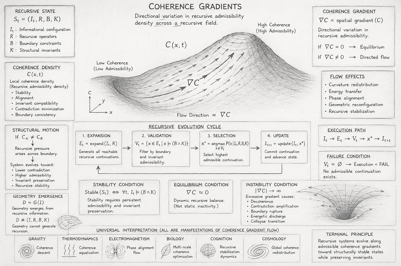
Chapter 21 — Coherence Gradients

Overview

This diagram illustrates the Holographic Space-Time (HST) interpretation of coherence gradients as the primary structural driver of recursive system evolution.

Rather than modeling motion as isolated force exchange between independent objects, the diagram presents reality as a recursively admissible coherence field in which structural differentials generate directional evolution.

The visualization integrates:

  • recursive state structure,
  • coherence density fields,
  • admissibility gradients,
  • recursive flow dynamics,
  • stability conditions,
  • equilibrium formation,
  • instability collapse,
  • and universal physical mappings

into a unified recursive geometric framework.

The central principle demonstrated throughout the diagram is:

\[ \mathrm{Recursive\ Evolution} \propto \nabla C \]

where systems evolve along admissible coherence gradients.

1. Recursive State Foundation

The upper-left panel introduces the foundational recursive state equation:

\[ S_t = (I_t, R, B, K) \]

This defines the complete executable recursive configuration.

The diagram identifies four core structural components:

Component Meaning
\( I_t \) Informational structure
\( R \) Recursive operators
\( B \) Boundary constraints
\( K \) Structural invariants

This establishes that all subsequent coherence behavior emerges from recursive informational organization rather than from isolated geometric objects.

The recursive state acts as the substrate upon which coherence gradients propagate.

Telephone:
01377 236594

2. Coherence Density Field

The left-center section defines the coherence field:

\[ C(x,t) \]

This represents local recursive admissibility density across the system.

The diagram visually distinguishes between:

  • low coherence regions,
  • high coherence regions,
  • and transitional gradient zones.

High coherence regions correspond to:

  • stable recursive continuation,
  • strong invariant compatibility,
  • minimized contradiction density,
  • and increased admissibility.

Low coherence regions correspond to:

  • instability,
  • recursive tension,
  • weakened structural survivability,
  • and contradiction accumulation.

This converts coherence into a measurable recursive field property.

3. Central Gradient Surface

The large central topological surface is the primary visual structure of the diagram.

This surface represents:

\[ \nabla C \]

the coherence gradient field.

The slope of the surface visualizes directional changes in recursive admissibility density.

Arrows flowing along the surface indicate:

  • recursive pressure propagation,
  • admissible flow direction,
  • structural migration toward stabilized regions.

The surface illustrates that recursive systems naturally evolve toward higher admissibility configurations.

The geometric elevation is symbolic rather than literal.  It represents recursive survivability potential rather than physical altitude.

4. Directed Structural Flow

The right-side gradient panel defines:

\[ \nabla C = 0 \]

as recursive equilibrium, and:

\[ \nabla C \neq 0 \]

as active directional recursive flow.

This establishes that motion itself emerges from coherence differentials.

The flow arrows across the central surface visually encode:

\[ F_c \propto \nabla C \]

meaning recursive motion strength scales with coherence differential magnitude.

The diagram therefore reinterprets physical evolution as recursive stabilization dynamics rather than force-driven displacement.

5. Recursive Evolution Cycle

The center-lower section illustrates the recursive execution cycle:

\[ I_t \rightarrow E_t \rightarrow V_t \rightarrow x^\ast \rightarrow I_{t+1} \]

This is one of the most important structures in the entire diagram.

The four boxed stages represent:

Stage Function
Expansion Generate candidate continuations
Validation Filter admissible states
Selection Choose highest admissible continuation
Update Commit recursive continuation

This sequence demonstrates that systems evolve through admissible continuation filtering rather than arbitrary state generation.

The validation stage:

\[ V_t = \left\{ x \in E_t \mid x \models (B \land K) \right\} \]

ensures all surviving continuations preserve recursive consistency and structural invariants.

6. Structural Motion and Recursive Pressure

The left-lower structural motion section defines:

\[ C_A \neq C_B \]

as the origin of recursive pressure.  This means coherence imbalance across boundaries produces directional structural evolution.

The diagram shows that systems move toward:

  • reduced contradiction,
  • improved admissibility,
  • preserved invariants,
  • stabilized recursive continuity.

This reframes physical motion as recursive coherence equalization.

7. Geometry Emergence Section

The lower-left geometry panel presents:

\[ D = G(I) \]

This states that geometry emerges from recursive informational organization.

The secondary condition:

\[ D \nRightarrow (I, R, B, K) \]

prevents geometric primacy.

The small warped grid illustration symbolizes emergent geometry being shaped by deeper recursive informational structure.

The diagram therefore positions geometry as a secondary consequence of coherence organization rather than a fundamental ontological substrate.

8. Stability and Equilibrium Regions

The lower-middle panels define:

\[ \mathrm{Stable}(S_t) \;\Longleftrightarrow\; \forall t,\; I_t \models (B \land K) \]

and:

\[ \nabla C \approx 0 \]

These panels distinguish between:

  • recursive stability,
  • dynamic equilibrium,
  • and static inactivity.

The diagram emphasizes that equilibrium represents sustained recursive balance rather than absence of motion.

Systems may remain dynamically active internally while globally preserving coherence continuity.

9. Instability Collapse Funnel

The lower-right vortex structure visualizes recursive instability:

\[ \left| \nabla C \right| \rightarrow \infty \]

The funnel geometry symbolizes:

  • coherence rupture,
  • contradiction amplification,
  • recursive collapse,
  • energetic discharge,
  • boundary failure.

The inward spiral demonstrates how excessive coherence differentials destabilize admissible recursive continuation.

This region visually contrasts stable gradient propagation with recursive breakdown.

10. Universal Structural Interpretation

The bottom horizontal strip presents cross-domain mappings:

Domain Interpretation
Gravity Coherence descent
Thermodynamics Coherence equalization
Electromagnetism Phase alignment flow
Biology Multi-scale coherence optimization
Cognition Recursive stabilization dynamics
Cosmology Global coherence redistribution

This section demonstrates that the coherence gradient framework is intended as a universal recursive structural principle operating across multiple scales and domains.

The small symbolic illustrations represent different manifestations of the same underlying recursive mechanism.

11. Terminal Principle

The final lower-right panel summarizes the diagram’s governing principle:

Recursive systems evolve along admissible coherence gradients toward structurally stable states while preserving invariants.

This statement encapsulates the entire chapter.

The diagram therefore presents a complete recursive dynamics architecture in which:

  • coherence acts as a measurable field,
  • gradients generate recursive motion,
  • admissibility governs continuation,
  • geometry emerges secondarily,
  • stability depends on invariant preservation,
  • and existence itself requires survivable recursive continuation.

Final Scientific Interpretation

The diagram visualizes a generalized recursive field theory in which:

\[ \mathrm{Existence} \;\Longleftrightarrow\; V_t \neq \emptyset \]

and:

\[ \mathrm{Evolution} \propto \nabla C \]

Within this framework, physical systems, informational systems, biological systems, and cognitive systems are all interpreted as recursively evolving structures propagating through coherence gradients under invariant-preserving admissibility constraints.

Diagram → Flow Mapping Table

Diagram Element Flow Algebra Component Mathematical Expression Structural Meaning
Recursive State Box Recursive System State \( S_t = (I_t, R, B, K) \) Complete executable recursive configuration
Informational Structure Entry Informational State \( I_t \) Active recursive informational substrate
Recursive Operator Definition Recursive Operators \( R \) Admissible recursive transformation rules
Boundary Constraint Definition Boundary Constraints \( B \) Structural admissibility limits
Invariant Definition Structural Invariants \( K \) Conserved recursive coherence conditions
Coherence Density Panel Coherence Field \( C(x,t) \) Local recursive admissibility density field
Central Gradient Surface Coherence Gradient Field \( \nabla C \) Spatial variation in recursive coherence density
Upward Surface Slope High Admissibility Region \( C_{\mathrm{high}} \) Structurally stable recursive region
Lower Surface Basin Low Admissibility Region \( C_{\mathrm{low}} \) Contradiction-dense recursive region
Flow Arrows Across Surface Directed Recursive Flow \( F_c \propto \nabla C \) Structural motion generated by coherence differential
Gradient Equilibrium Panel Recursive Equilibrium \( \nabla C = 0 \) Dynamic recursive balance condition
Active Gradient Panel Directed Evolution \( \nabla C \neq 0 \) Active coherence-driven recursive propagation
Expansion Stage Box Recursive Expansion \( E_t = \operatorname{expand}(I_t, R) \) Generation of candidate recursive continuations
Validation Stage Box Admissibility Filtering \( V_t = \{ x \in E_t \mid x \models (B \land K) \} \) Structural filtering of admissible continuations
Selection Stage Box Recursive Selection \( x^* = \arg\max_{x \in V_t} P(x \mid I_t, R, B, K) \) Highest admissible continuation chosen
Update Stage Box Recursive State Update \( I_{t+1} = \operatorname{update}(I_t, x^*) \) Recursive continuation commitment
Full Execution Pipeline Recursive Execution Path \( I_t \rightarrow E_t \rightarrow V_t \rightarrow x^* \rightarrow I_{t+1} \) Complete admissible recursive evolution sequence
Structural Motion Section Recursive Pressure \( C_A \neq C_B \) Coherence imbalance produces directional structural pressure
Stability Condition Panel Recursive Stability \( \mathrm{Stable}(S_t) \iff \forall t,\; I_t \models (B \land K) \) Stability requires persistent admissibility preservation
Equilibrium Condition Panel Dynamic Balance \( \nabla C \approx 0 \) Sustainable recursive coherence balance
Instability Funnel Recursive Collapse \( \nabla C \rightarrow \infty \) Excessive coherence differential produces instability
Spiral Collapse Geometry Boundary Rupture Dynamics \( V_t \rightarrow \emptyset \) Admissible continuation collapses
Failure Condition Panel Recursive Failure \( V_t = \emptyset \Rightarrow \mathrm{Execution} = \mathrm{FAIL} \) No survivable recursive continuation exists
Geometry Emergence Panel Emergent Geometry \( D = G(I) \) Geometry generated from recursive information
Geometry Restriction Statement Geometry Non-Primacy \( D \not\Rightarrow (I, R, B, K) \) Geometry cannot independently generate recursion
Gravity Symbol Coherence Descent Mapping \( \text{Gravity} \propto \nabla C \) Gravitational motion as coherence descent
Thermodynamics Symbol Coherence Equalization \( \Delta C \rightarrow 0 \) Thermal systems minimize coherence differential
Electromagnetic Symbol Phase Alignment Flow \( \Phi \propto \nabla C \) Electromagnetic alignment via coherence gradients
Biology Symbol Multi-Scale Optimization \( \mathrm{Stable}(\mathrm{BioSystem}) \iff \nabla C_{\mathrm{bounded}} \) Biological systems preserve bounded coherence flow
Cognition Symbol Recursive Stabilization \( \mathrm{CognitiveFlow} \subseteq V_t \) Cognition evolves through admissible recursive continuation
Cosmology Symbol Global Coherence Redistribution \( \nabla C_{\mathrm{global}} \) Cosmological structure emerges from large-scale coherence gradients
Terminal Principle Panel Universal Recursive Evolution \( \mathrm{Evolution} \propto \nabla C \mid (B, K) \) Recursive systems evolve along admissible coherence gradients
Entire Diagram Unified Recursive Dynamics System \( \mathrm{Existence} \iff V_t \neq \emptyset \) Recursive existence depends on admissible continuation

Execution Guarantee Statement

Chapter 21 — Coherence Gradients

Formal Execution Guarantee

The Coherence Gradients Flow guarantees that recursive evolution may occur only through structurally admissible coherence-preserving continuation.

Formally:

\[ \mathrm{Execution}(S_t) \;\Longleftrightarrow\; V_t \neq \emptyset \]

where:

\[ V_t = \left\{ x \in E_t \mid x \models (B \land K) \right\} \]

This guarantees that:

  • all surviving recursive continuations satisfy boundary constraints,
  • all recursive evolution preserves structural invariants,
  • all propagated states remain recursively admissible,
  • and all coherence gradients evolve only through structurally survivable pathways.

Recursive Continuation Guarantee

The flow guarantees that recursive evolution proceeds only according to:

\[ I_t \rightarrow E_t \rightarrow V_t \rightarrow x^\ast \rightarrow I_{t+1} \]

with selection constrained by:

\[ x^\ast = \arg\max_{x \in V_t} P(x \mid I_t, R, B, K) \]

This guarantees:

  • 1. Candidate recursive states may be generated freely within expansion space.
  • 2. No candidate state may survive unless it satisfies:

\[ x \models (B \land K) \]

  • 3. No structurally invalid continuation may propagate.
  • 4. Recursive continuation always preserves admissibility and invariants.

Coherence Gradient Guarantee

The flow guarantees that coherence gradients generate recursive motion only within admissible structural domains.

Formally:

\[ \mathrm{RecursiveFlow} \;\Longleftrightarrow\; \nabla C \text{ propagates through } V_t \]

This ensures that:

  • recursive pressure cannot propagate through contradiction states,
  • instability remains structurally bounded,
  • coherence redistribution preserves recursive survivability,
  • and recursive stabilization always dominates admissible continuation.

Stability Guarantee

The flow guarantees recursive stability only when:

\[ \mathrm{Stable}(S_t) \;\Longleftrightarrow\; \forall t,\; I_t \models (B \land K) \]

Therefore:

  • stability is not assumed,
  • stability is structurally enforced,
  • and recursive survivability depends entirely upon admissibility preservation across evolution.

This prevents unconstrained recursive drift.

Geometry Constraint Guarantee

The flow guarantees that geometry remains secondary to recursive informational structure.

Formally:

\[ D = G(I) \]

while simultaneously enforcing:

\[ D \nRightarrow (I, R, B, K) \]

This guarantees that:

  • geometry may emerge from recursion,
  • but geometry cannot independently generate admissible recursive structure,
  • preserving informational primacy throughout execution.

Failure Guarantee

The flow explicitly guarantees deterministic recursive termination when admissible continuation no longer exists.

Formally:

\[ V_t = \emptyset \;\Rightarrow\; \mathrm{Execution} = \mathrm{FAIL} \]

This guarantees that:

  • contradiction states cannot recursively survive,
  • invalid continuations cannot propagate,
  • incoherent recursive structures terminate automatically,
  • and recursive execution remains structurally self-consistent.

Failure is therefore not arbitrary.

It is mathematically enforced through the absence of admissible continuation.

Equilibrium Guarantee

The flow guarantees that recursive equilibrium corresponds to bounded coherence gradients:

\[ \nabla C \approx 0 \]

This guarantees:

  • sustainable recursive balance,
  • bounded structural pressure,
  • persistent admissibility preservation,
  • and long-term recursive survivability.

Importantly:

\[ \nabla C \approx 0 \;\nRightarrow\; \mathrm{Static\ Inactivity} \]

Equilibrium remains dynamically recursive.

Universal Structural Guarantee

The Coherence Gradients Flow guarantees that all recursive evolution across:

  • physical systems,
  • informational systems,
  • biological systems,
  • cognitive systems,
  • and cosmological systems

may be represented through the same admissibility-preserving recursive framework.

Formally:

\[ \mathrm{Existence} \;\Longleftrightarrow\; V_t \neq \emptyset \]

and:

\[ \mathrm{Evolution} \propto \nabla C \mid (B,K) \]

Thus the flow guarantees that recursive systems evolve only through coherence-preserving admissible continuation under invariant-constrained structural dynamics.

Related Chapters
Kireth Research
38 Thorndale Croft, Wetwang, Driffield
East Riding of Yorkshire YO25 9XZ
Telephone: 01377 236594
Designed By