Chapter 36
Field Lines as Gradient Paths

PART III — Electromagnetism & Field Structure
Author: Mark Higgins
© Mark Anthony Higgins 11 October 2025
Revised Date: 09 June 2026
Audio Overview

36.1 Introduction

Field lines are among the most recognizable visual tools in physics. From electric and magnetic fields to gravitational potentials and fluid flows, field lines provide a geometric representation of how forces and influences propagate through space. They appear in textbooks as arrows emerging from charges, looping around magnets, or converging toward masses, giving an intuitive picture of otherwise invisible phenomena.

Despite their usefulness, conventional physics generally treats field lines as mathematical constructs rather than physical entities. They are considered visualization aids that represent solutions to differential equations, not structures that possess independent ontological significance. The field exists; the lines merely illustrate its direction and magnitude.

Within the Holographic Space-Time (HST) framework, a different interpretation emerges.

Field lines are not arbitrary drawings imposed upon a field after the fact. Instead, they arise naturally as observable traces of underlying coherence gradients. They represent preferred paths through curvature space along which coherence tension is redistributed. What appears as a field line is therefore the geometric manifestation of a deeper optimization process occurring within the boundary structure of reality itself.

In HST, fields emerge from coherence imbalances. Whenever coherence density varies across a region, curvature gradients form. These gradients create directional pathways that guide energy transfer, information propagation, and structural realignment. The resulting trajectories are observed macroscopically as field lines.

Thus, field lines are reinterpreted not as symbolic representations but as emergent geometric pathways generated by the structure of coherence gradients.

36.2 The Conventional View of Field Lines

In classical field theory, field lines are defined by the local direction of a vector field.

For an electric field:
the field line at any point follows the direction of the electric field vector.

Similarly, for gravity:
the field line follows the gradient of the gravitational potential.

These constructions provide useful visualizations and predictive tools. Objects accelerate along directions determined by these gradients, and field lines illustrate the resulting motion.

However, conventional theory typically leaves unanswered a deeper question:

Why should these gradients exist in the particular forms observed?

The equations describe the gradients but do not provide a geometric mechanism explaining why nature organizes itself into these directional structures.

HST addresses this question by tracing field formation back to coherence distributions and boundary dynamics.

36.3 Coherence Gradients as the Origin of Fields

Within HST, every physical system possesses a coherence distribution:

\[ C(x,y,z,t) \]

which defines how structural alignment is organized across a region of space.

Perfectly uniform coherence produces no preferred direction.

However, when coherence varies spatially, a gradient emerges:

\[ \nabla C \]

This gradient represents an imbalance in boundary organization.

Regions of high coherence and low coherence create tension across the field structure. The system naturally seeks configurations that reduce these tensions while preserving global coherence conservation.

As a result, directional pathways emerge.

These pathways correspond to routes along which coherence redistribution can occur most efficiently.

The observable field is therefore not fundamental.

It is the macroscopic consequence of coherence-gradient optimization.

36.4 Field Lines as Geodesics of Coherence

In differential geometry, geodesics represent the shortest or most stable paths through a curved space.

HST extends this concept.

Field lines become coherence geodesics.

Rather than minimizing spatial distance, they minimize coherence tension.

A field line therefore follows the direction of greatest coherence descent:

Objects interacting with the field naturally follow these trajectories because movement away from them requires additional coherence expenditure.

The familiar curved shapes observed around charges, magnets, and massive bodies therefore emerge as stable pathways through coherence geometry.

What physicists traditionally call a field line becomes, in HST language, a gradient path through a coherence landscape.

36.5 Why Field Lines Never Cross

One of the most familiar rules in physics is that field lines cannot intersect.

Conventionally this follows from vector field mathematics: two different field directions cannot simultaneously exist at the same point.

HST provides a structural interpretation.

If two coherence-gradient paths intersected while maintaining independent directional definitions, the same region would require multiple incompatible curvature states simultaneously.

Such a configuration would violate coherence stability.

The system therefore resolves toward a single locally stable gradient direction.

As a consequence:

  • Field lines remain non-intersecting.
  • Coherence flow remains well-defined.
  • Curvature evolution remains deterministic.
  • Boundary stability is preserved.

The non-crossing rule emerges as a direct consequence of coherence consistency.

36.6 Energy Flow Along Gradient Paths

Field lines are not merely geometric features.

They also define preferred transport routes.

Whenever energy propagates through a field, it tends to follow existing coherence gradients because these paths minimize structural resistance.

This explains why:

  • Electric currents follow electric field structures.
  • Gravitational motion follows gravitational gradients.
  • Electromagnetic radiation propagates through field geometry.
  • Information transfer exhibits directional bias.

In HST, energy transport and coherence transport become two descriptions of the same underlying process.

Energy moves where coherence gradients permit efficient redistribution.

36.7 Emergent Geometry and Field Structure

The shapes of field lines reveal information about the underlying coherence landscape.

Straight field lines indicate approximately uniform gradients.

Curved field lines indicate varying coherence densities.

Converging field lines indicate coherence sinks.

Diverging field lines indicate coherence sources.

Closed field loops indicate stable self-contained coherence circulation.

The geometry of field structures therefore becomes a direct diagnostic tool for understanding the hidden coherence topology beneath observable phenomena.

Field line patterns are effectively maps of the curvature architecture from which physical interactions emerge.

36.8 HST Interpretation

Within Holographic Space-Time theory, field lines are reinterpreted as gradient paths generated by coherence-density variation across boundary structures.

They are not merely visualization tools.

They are emergent geometric trajectories formed as the system minimizes coherence tension while maintaining structural stability.

In this view:

  • Coherence gradients generate curvature.
  • Curvature generates field structure.
  • Field structure generates gradient paths.
  • Gradient paths appear observationally as field lines.
  • Matter and energy follow these paths because they represent stable routes through coherence geometry.

Field lines therefore become observable traces of the deeper coherence architecture of reality.

Rather than being mathematical conveniences drawn onto fields, they are the visible footprints of the geometric processes through which boundary coherence organizes the universe.

flow "HST_FieldLines_as_GradientPaths" v1.0

  authors:
    - Mark Higgins
    - Sky

  chapter:
    number: 36
    title: "Field Lines as Gradient Paths"

  purpose:
    Define field lines as emergent gradient paths produced by
    coherence-density variation, boundary tension, and curvature
    alignment within Holographic Space-Time.

  system:
    name: FieldLineGradientSystem
    type: HST_Field_Geometry_Model

  inputs:

    I_t:
      description: Physical system state at time t

      contains:
        - boundary_structure B_t
        - coherence_distribution C_t
        - curvature_configuration K_t
        - field_region R_t

  state_variables:

    C_t:
      description: Coherence distribution across the field region

    grad_C_t:
      symbol: ∇C_t
      description: Spatial coherence gradient

    T_t:
      description: Boundary tension generated by coherence mismatch

    K_t:
      description: Curvature configuration induced by coherence imbalance

    F_t:
      description: Emergent field state

    L_t:
      description: Field line path set

    P_t:
      description: Preferred gradient path through coherence geometry

  parameters:

    C_min:
      description: Minimum coherence required for stable field formation

    T_max:
      description: Maximum permitted unresolved boundary tension

    epsilon:
      description: Local tolerance for gradient-path stability

  process:

    step_1:

      name: Map_Coherence_Distribution

      input:
        - I_t

      operation:
        extract_coherence_geometry

      output:
        - C_t

    step_2:

      name: Detect_Coherence_Gradient

      input:
        - C_t

      operation:
        compute_spatial_gradient

      equation:
        grad_C_t = ∇C_t

      output:
        - grad_C_t

    step_3:

      name: Generate_Boundary_Tension

      input:
        - grad_C_t

      operation:
        convert_gradient_to_boundary_tension

      equation:
        T_t = Φ(∇C_t)

      output:
        - T_t

    step_4:

      name: Induce_Curvature_Configuration

      input:
        - C_t
        - T_t

      operation:
        resolve_tension_into_curvature

      equation:
        K_t = Ψ(C_t,T_t)

      output:
        - K_t

    step_5:

      name: Form_Field_State

      input:
        - K_t
        - grad_C_t

      operation:
        generate_emergent_field

      equation:
        F_t = Ω(K_t,∇C_t)

      output:
        - F_t

    step_6:

      name: Trace_Gradient_Paths

      input:
        - F_t
        - grad_C_t

      operation:
        follow_direction_of_coherence_descent

      equation:
        P_t ∝ -∇C_t

      output:
        - P_t

    step_7:

      name: Define_Field_Lines

      input:
        - P_t

      operation:
        stabilise_path_set

      equation:
        L_t = { P_t | P_t follows stable coherence gradient }

      output:
        - L_t

    step_8:

      name: Prevent_Path_Crossing

      input:
        - L_t

      operation:
        enforce_single_local_gradient_direction

      condition:
        ∀x ∈ R_t, direction(L_t at x) is unique

      output:
        - non_intersecting_field_lines

    step_9:

      name: Transport_Energy_Along_Paths

      input:
        - L_t
        - F_t

      operation:
        route_energy_through_minimum_resistance_gradient

      equation:
        E_flow,t → L_t

      output:
        - directed_energy_transport

  invariants:

    coherence_threshold:
      condition:
        C_t ≥ C_min

      meaning:
        Field structure remains coherent enough to form stable paths

    gradient_uniqueness:
      condition:
        ∀x ∈ R_t, ∇C_t has one stable resolved direction

      meaning:
        Field lines do not cross

    tension_limit:
      condition:
        T_t ≤ T_max

      meaning:
        Boundary tension remains resolvable

    field_path_stability:
      condition:
        |δP_t| ≤ epsilon

      meaning:
        Gradient path remains locally stable

    conservation:
      condition:
        Total_Coherence(t+1) = Total_Coherence(t)

      meaning:
        Field-line formation redistributes coherence rather than
        creating or destroying it

  execution:

    valid_case:

      if:
        - C_t ≥ C_min
        - T_t ≤ T_max
        - ∇C_t is defined
        - local_gradient_direction is unique

      then:
        - K_t forms
        - F_t emerges
        - P_t follows -∇C_t
        - L_t becomes stable field-line geometry
        - Execution_State = STABLE

    failure_case:

      if:
        - C_t < C_min
        - T_t > T_max
        - ∇C_t undefined
        - multiple incompatible local directions exist

      then:
        - field_path becomes unstable
        - boundary coherence deforms or collapses
        - Execution_State = FAIL_OR_RECONFIGURE

  output:

    S_t+1:

      description:
        Updated physical state containing stable field-line geometry

      contains:
        - updated_coherence_distribution C_t+1
        - resolved_curvature_configuration K_t+1
        - emergent_field_state F_t+1
        - stable_field_line_paths L_t+1

  summary:

    Field lines are not independent physical objects or arbitrary
    visual aids. In HST they are stable gradient paths produced by
    coherence-density variation, boundary tension, and curvature
    resolution. Matter, energy, and information follow these paths
    because they represent locally stable routes through coherence
    geometry.

What This Flow Implements

Overview

This flow implements the Holographic Space-Time (HST) interpretation of field-line formation as an emergent consequence of coherence-density gradients, boundary tension, and curvature organization. Rather than treating field lines as purely mathematical visualization tools, the flow formalizes them as physically meaningful gradient paths through coherence geometry.

The implementation begins with a coherence distribution existing across a spatial region. Variations within this distribution create gradients that generate boundary tension. The resulting tension induces curvature, which subsequently organizes into stable field structures. These structures define preferred trajectories through the system that appear observationally as field lines.

The flow therefore provides a complete causal chain linking coherence organization to observable field geometry.

Coherence Distribution Mapping

It → Ct

where:

Ct = CoherenceMap(It)

The coherence map represents the spatial organization of boundary-aligned information throughout the physical region under consideration.

Within HST, coherence is treated as a measurable structural property rather than an abstract quantity. Regions may possess differing coherence densities depending on local geometric organization.

This stage establishes the foundational information from which all subsequent field behavior emerges.

Gradient Detection

Once coherence has been mapped, the flow calculates its spatial variation.

Ct → ∇Ct

where:

∇Ct = Gradient(Ct)

The coherence gradient identifies how rapidly coherence changes from one location to another.

If coherence remains uniform:

∇Ct = 0

no preferred direction exists and no field structure emerges.

If coherence varies spatially:

∇Ct ≠ 0

directional asymmetry appears within the system.

This asymmetry forms the origin of all field-line behavior.

Boundary Tension Generation

The flow then converts coherence gradients into boundary tension.

∇Ct → Tt

where:

Tt = Φ(∇Ct)

Boundary tension represents unresolved coherence imbalance.

Large gradients correspond to stronger tension.

Small gradients correspond to weaker tension.

This stage provides the physical mechanism through which coherence differences acquire dynamical significance.

Rather than postulating forces directly, HST interprets force-producing behavior as arising from tension generated by coherence mismatch.

Curvature Formation

The generated tension reorganizes local geometry.

(Ct,Tt) → Kt

where:

Kt = Ψ(Ct,Tt)

Curvature acts as the geometric response to coherence imbalance.

The flow therefore treats curvature not as a fundamental object but as a consequence of coherence-driven tension resolution.

Regions with greater tension produce stronger curvature effects.

Regions approaching coherence equilibrium produce weaker curvature effects.

This stage establishes the geometric substrate from which fields emerge.

Field Emergence

Once curvature has formed, a field state becomes observable.

(Kt,∇Ct) → Ft

where:

Ft = Ω(Kt,∇Ct)

The field is therefore not fundamental within HST.

Instead, it emerges from the interaction between curvature organization and coherence gradients.

Traditional electric, magnetic, and gravitational fields become different manifestations of the same underlying coherence-curvature mechanism.

Gradient Path Construction

The flow next determines the preferred trajectories through the field.

Ft → Pt

where:

Pt ∝ -∇Ct

The negative sign indicates movement toward reduced coherence tension.

These paths represent the most stable routes available within the coherence landscape.

In HST terminology, these are coherence geodesics.

They define how the system naturally redistributes information, energy, and structural alignment.

Field-Line Formation

Stable gradient paths are collected into a coherent field-line geometry.

Pt → Lt

where:

Lt = {Pt | Pt follows stable coherence gradient}

The resulting field lines are not arbitrary graphical constructions.

They are emergent geometric trajectories that encode the organization of the underlying coherence field.

Field-line shape therefore becomes a direct reflection of coherence topology.

Non-Crossing Constraint

The flow enforces a unique local gradient direction.

Direction(Lt,x) = Unique

for every point within the field region.

This implementation reproduces the well-known physical observation that field lines do not intersect.

Within HST, the reason is structural rather than merely mathematical.

Crossing field lines would require multiple incompatible coherence-gradient directions to occupy the same location simultaneously.

Such a state would violate coherence stability and therefore cannot persist.

The flow automatically prevents these configurations.

Energy Transport Along Field Lines

The final operational stage implements transport.

Eflow,t → Lt

Energy propagates preferentially along established coherence-gradient paths.

This reproduces the observed tendency of physical systems to move along field structures rather than arbitrary trajectories.

Within HST, energy flow and coherence redistribution become different descriptions of the same process.

Field lines therefore function as transport channels through coherence geometry.

Conservation Mechanism

The flow enforces coherence conservation through the invariant:

TotalCoherence(t+1)
=
TotalCoherence(t)

Field formation does not create coherence.

Field formation does not destroy coherence.

Instead, coherence is redistributed through geometric reorganization.

This mirrors conservation principles found throughout conventional physics while providing a deeper structural interpretation.

Scientific Interpretation

The complete implementation formalizes the following causal chain:

Coherence Distribution
        ↓
Coherence Gradient
        ↓
Boundary Tension
        ↓
Curvature Formation
        ↓
Field Emergence
        ↓
Gradient Path Formation
        ↓
Field-Line Geometry
        ↓
Energy Transport

Within the HST framework, field lines are therefore interpreted as observable manifestations of coherence gradients acting through curvature geometry.

They are neither fundamental objects nor mere visualization tools.

They are emergent structures generated by the system's attempt to minimize coherence tension while preserving global stability.

The flow demonstrates how field-line geometry can arise naturally from coherence organization alone, providing a unified explanation for the directional structure observed throughout electromagnetic, gravitational, and other field phenomena.

How to Read This Flow

Purpose of This Flow

This flow describes how field lines emerge from coherence gradients within the Holographic Space-Time (HST) framework. It provides a complete structural pathway linking coherence organization to the observable field geometries found throughout physics.

In conventional physics, field lines are typically viewed as graphical representations of vector fields. They illustrate direction and magnitude but are not generally considered physical structures themselves.

Within HST, field lines are interpreted differently.

They are treated as stable gradient trajectories generated by coherence-density variation across a boundary-defined geometric system. The flow formalizes how these trajectories emerge, stabilize, and guide energy transport.

The purpose of this section is to explain how each stage of the flow contributes to the formation of observable field-line geometry.

Reading the Flow as a Causal Chain

The entire flow can be summarized as:

It
→ Ct
→ ∇Ct
→ Tt
→ Kt
→ Ft
→ Pt
→ Lt
→ St+1

This sequence should not be viewed as computer code.

It is a causal description of how physical structure evolves.

Each stage produces the conditions necessary for the next stage to exist.

The flow therefore describes a physical transformation sequence rather than a software execution sequence

Step 1 — Initial Physical State

The flow begins with:

It

representing the complete physical state of the system.

The input state contains:

It = (Bt, Ct, Kt, Rt)

where:

Symbol Meaning
Bt Boundary Structure
Ct Coherence Distribution
Kt Curvature Configuration
Rt Field Region

Step 2 — Coherence Mapping

The first transformation is:

It → Ct

where:

Ct = CoherenceMap(It)

This operation extracts the coherence structure embedded within the physical system.

When reading this stage, imagine constructing a complete map of how organized the system is at every location.

Regions may contain:

  • High coherence
  • Moderate coherence
  • Low coherence

The resulting map becomes the foundation of all later field behavior.

Without coherence variation, no field lines can emerge.

Step 3 — Gradient Detection

The next stage is:

Ct → ∇Ct

where:

∇Ct = Gradient(Ct)

The gradient measures how coherence changes across space.

This is one of the most important stages in the entire flow.

A gradient identifies:

  • Direction of greatest change
  • Magnitude of change
  • Spatial asymmetry

When reading this stage, imagine a landscape of hills and valleys.

The gradient indicates the steepest slope.

In HST, field lines ultimately emerge from these slopes.

No gradient means:

∇Ct = 0

No preferred direction exists.

No field structure forms.

Step 4 — Boundary Tension Formation

The flow then generates tension:

∇Ct → Tt

where:

Tt = Φ(∇Ct)

This stage converts coherence imbalance into physical tension.

When coherence differs between neighboring regions, the boundary between them becomes strained.

The larger the gradient:

|∇Ct|

the larger the tension.

When reading this section, think of a stretched membrane.

Differences in tension create forces that attempt to restore stability.

Within HST, boundary tension acts as the engine driving field formation.

Telephone:
01377 236594

Step 5 — Curvature Generation

The next stage is:

(Ct,Tt) → Kt

where:

Kt = Ψ(Ct,Tt)

Curvature emerges as the geometric response to tension.

This stage explains how coherence imbalance reshapes geometry.

When reading this step, imagine a flat elastic sheet.

Applying tension causes the sheet to bend.

Similarly, coherence tension generates curvature within the underlying field structure.

The greater the unresolved tension, the greater the curvature response.

Step 6 — Field Emergence

The flow now produces a field:

(Kt,∇Ct) → Ft

where:

Ft = Ω(Kt,∇Ct)

This stage is critical.

Within HST, fields do not exist independently.

They emerge from:

  • Coherence gradients
  • Boundary tension
  • Curvature organization

The field therefore represents a higher-level manifestation of deeper geometric processes.

When reading this stage, think of the field as the visible expression of hidden coherence structure.

Step 7 — Gradient Path Formation

The flow then identifies preferred trajectories:

Ft → Pt

where:

Pt ∝ -∇Ct

This equation states that stable motion follows the direction of decreasing coherence tension.

The path seeks regions of greater stability.

When reading this stage, imagine water flowing downhill.

The water naturally follows the steepest descent.
Likewise, coherence seeks routes that reduce imbalance.

These routes become the fundamental building blocks of field lines.

Step 8 — Field-Line Construction

The next stage constructs the field-line network:

Pt → Lt

where:

Lt = {Pt | Pt follows stable coherence gradient}

At this point, individual paths become an organized geometric structure.

The collection of stable paths forms the observable field-line pattern.

When reading this stage, imagine drawing every stable route across a landscape.

The complete collection reveals the underlying geometry.

This is exactly what field lines represent in HST.

Step 9 — Non-Crossing Enforcement

The flow then applies a stability constraint:

Direction(Lt,x) = Unique

for every location:

x ∈ Rt

This prevents multiple incompatible directions from occupying the same point.

When reading this stage, remember that a coherence gradient defines a single locally stable direction.

Two different directions cannot simultaneously describe the same local gradient.

As a result:

  • Field lines do not intersect.
  • Direction remains well-defined.
  • Coherence remains stable.

The familiar non-crossing property of field lines emerges naturally.

Step 10 — Energy Transport

The final operational stage is:

Eflow,t → Lt

This describes energy moving along established gradient paths.

When reading this stage, interpret field lines as transport channels.

Energy follows these routes because they represent minimum-resistance pathways through coherence geometry.

This explains why physical motion frequently aligns with field structure.

Matter, radiation, and information all preferentially propagate along stable coherence gradients.

Reading the Invariants

The invariant section defines conditions that must remain true throughout execution.

For example:

Ct ≥ Cmin

means coherence must remain above the minimum stability threshold.

Likewise:

Tt ≤ Tmax

ensures boundary tension remains physically resolvable.

The uniqueness condition:

∀x ∈ Rt :
Direction(Lt,x) = Unique

guarantees that field lines remain non-crossing.

These invariants act as stability laws governing the entire process.

Reading the Success Conditions

The flow executes successfully when:

Ct ≥ Cmin
Tt ≤ Tmax
∇Ct exists
UniqueGradientDirection = TRUE

When these conditions are satisfied:

Kt forms
Ft emerges
Pt follows -∇Ct
Lt stabilises

The resulting field-line geometry becomes physically meaningful and stable.

Reading the Failure Conditions

The failure conditions identify situations where field-line formation cannot remain stable.

Examples include:

Ct < Cmin

or

Tt > Tmax

or

∇Ct undefined

Under these conditions:

Execution(St) = FAIL_OR_RECONFIGURE

The system must reorganize its coherence structure before stable field lines can exist.

Scientific Interpretation

The flow should ultimately be read as a geometric emergence process:

Coherence
      ↓
Gradient
      ↓
Tension
      ↓
Curvature
      ↓
Field
      ↓
Path
      ↓
Field Line
      ↓
Energy Transport

Every stage follows naturally from the one before it.

The flow therefore provides a complete HST description of how field lines emerge from coherence geometry.

Rather than being abstract mathematical drawings placed onto a field after the fact, field lines become physically meaningful gradient paths generated by the system's continual attempt to minimize coherence tension while preserving structural stability.

Flow → Equation Tri-Mapping Table

Flow Layer HST Equation Layer Physical Interpretation
Physical State Initialization I_t = (B_t,C_t,K_t,R_t) Complete boundary, coherence, curvature, and field-region state
Coherence Mapping C_t = CoherenceMap(I_t) Extract spatial coherence structure
Gradient Detection ∇C_t = Gradient(C_t) Measure coherence variation across space
Uniform-State Condition ∇C_t = 0 No preferred direction exists
Gradient-State Condition ∇C_t ≠ 0 Directional asymmetry exists
Boundary Tension Formation T_t = Φ(∇C_t) Coherence imbalance generates boundary tension
Tension Magnitude Scaling T_t ∝ ∇C_t Larger gradients produce larger tension
Curvature Generation K_t = Ψ(C_t,T_t) Tension resolves into curvature geometry
Curvature Scaling K_t ∝ T_t Stronger tension generates stronger curvature
Field Emergence F_t = Ω(K_t,∇C_t) Curvature and gradients produce observable fields
Gradient Path Construction P_t ∝ -∇C_t Stable trajectories follow coherence descent
Geodesic Condition δP_t → 0 Path approaches local stability
Field-Line Formation L_t = {P_t | P_t stable} Stable gradient paths become field lines
Local Direction Constraint ∀x ∈ R_t, Direction(L_t,x)=Unique Single stable field direction per location
Non-Crossing Condition ∄x:(L_i ∩ L_j)_x, i ≠ j Field lines cannot intersect
Energy Routing E_flow,t → L_t Energy propagates along field lines
Information Routing I_flow,t → L_t Information follows coherence pathways
Transport Efficiency min(ΔT_t) Paths minimise coherence tension
Coherence Threshold C_t ≥ C_min Minimum coherence required for field stability
Tension Constraint T_t ≤ T_max Boundary tension remains resolvable
Path Stability Constraint δP_t ≤ ε Field trajectory remains stable
Field Stability Condition F_t ≠ ∅ Emergent field remains defined
Conservation Invariant C_total(t+1)=C_total(t) Coherence is redistributed, not created
Stable Execution Execution(S_t)=STABLE Field-line geometry successfully forms
Failure Condition C_t < C_min Insufficient coherence for field formation
Failure Condition T_t > T_max Excessive unresolved boundary tension
Failure Condition ∇C_t undefined No valid gradient structure exists
Failure Condition ∃x: MultipleDirections(x) Competing gradient directions destabilise geometry
Reconfiguration State Execution(S_t)=FAIL_OR_RECONFIGURE System must reorganise before stable field lines can exist
Complete Flow Chain I_t → C_t → ∇C_t → T_t → K_t → F_t → P_t → L_t → S_t+1 Full HST field-line emergence sequence
HST Core Relation ∇C_t → T_t → K_t → F_t → L_t Coherence gradients generate observable field-line geometry
Physical Interpretation L_t ≡ Stable Coherence Geodesics Field lines are gradient paths through coherence geometry
Chapter Summary Field Lines ∝ -∇C_t Observable field structure emerges from coherence-gradient descent pathways

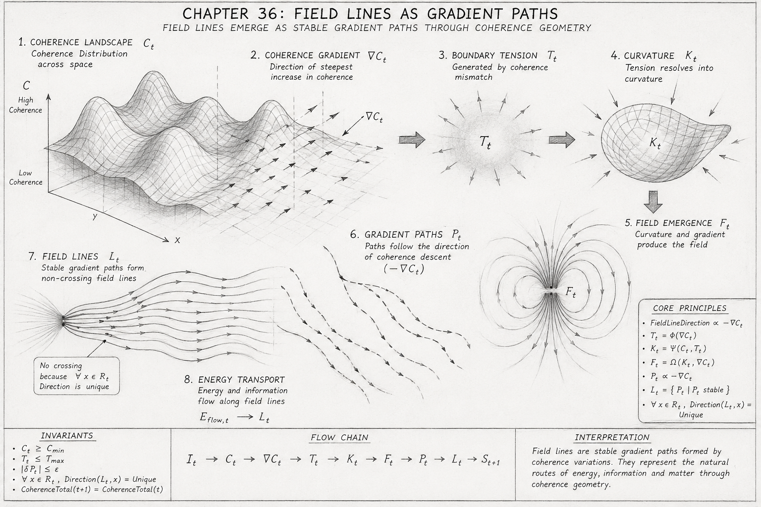
Chapter 36 — Field Lines as Gradient Paths

Overview

This diagram illustrates the Holographic Space-Time (HST) interpretation of field lines as emergent gradient paths formed through coherence geometry. Rather than viewing field lines as merely graphical representations of vector fields, the diagram presents them as physically meaningful trajectories generated by coherence gradients, boundary tension, and curvature organization.

The figure traces the complete causal chain from coherence distribution through field formation and ultimately to energy transport, showing how observable field structures emerge naturally from underlying coherence dynamics.

Stage 1 — Coherence Landscape

The left-hand side of the diagram begins with the coherence landscape CtC_t.

The surface represents spatial variations in coherence density across a physical region.

High elevations correspond to regions of greater coherence concentration.

Lower regions correspond to reduced coherence density.

Unlike conventional field theory, which begins with an already-existing field, HST begins with coherence organization itself.

The landscape therefore serves as the foundational structure from which all subsequent field behavior emerges.

The peaks and valleys illustrate that coherence is not uniformly distributed throughout space.

These variations are the origin of directional structure.

Stage 2 — Coherence Gradient Formation

The next section illustrates the coherence gradient:

\[ \nabla C_t \]

The arrows superimposed on the landscape indicate the direction of greatest coherence variation.

This stage identifies the local geometric asymmetries present within the coherence field.

In HST, gradients represent more than mathematical derivatives.

They define physically meaningful directional biases within the underlying coherence structure.

The gradient field determines where coherence imbalance exists and therefore where boundary tension will arise.

Without gradients:

\[ \nabla C_t = 0 \]

no preferred direction exists and field lines cannot form.

Stage 3 — Boundary Tension Generation

The central tension region represents:

\[ T_t \]

Boundary tension emerges whenever neighboring regions possess different coherence densities.

The radiating arrows illustrate unresolved structural imbalance.

This stage translates coherence variation into a dynamical quantity capable of driving geometric change.

Within HST, tension acts as the intermediary between coherence organization and curvature formation.

The stronger the coherence gradient, the greater the resulting tension.

The diagram depicts this as a concentrated source region from which geometric responses originate.

Stage 4 — Curvature Formation

The bowl-shaped geometric structure represents:

\[ K_t \]

Curvature is shown as the direct response to boundary tension.

The mesh surface visually demonstrates how geometry deforms under coherence-induced stress.

This section illustrates one of the central principles of HST:

Curvature is not fundamental.

Instead, curvature emerges from the system's attempt to resolve coherence imbalance.

The arrows converging toward the curvature surface indicate the continual influence of boundary tension on geometric structure.

The shape itself symbolizes the transformation of tension into stable curvature geometry.

Stage 5 — Field Emergence

The next stage shows the formation of the observable field:

\[ F_t \]

The characteristic field pattern illustrates how curvature and coherence gradients combine to generate structured directional behavior.

Within the HST framework, fields are secondary phenomena.

They emerge from deeper geometric processes occurring within coherence space.

The diagram deliberately places field formation after curvature generation to emphasize this causal ordering.

Field structure is therefore interpreted as a manifestation of coherence-driven geometry rather than a fundamental ingredient of reality.

Stage 6 — Gradient Path Construction

The dashed trajectories labelled PtP_t represent gradient paths.

These paths follow:

\[ P_t \propto -\nabla C_t \]

The negative gradient indicates motion toward reduced coherence tension.

The trajectories illustrate how the system naturally selects routes that minimize instability.

In geometric terms, these are coherence geodesics.

The dashed style emphasizes that these paths emerge from the underlying coherence landscape rather than being externally imposed.

They represent the most stable routes available within the field geometry.

Stage 7 — Stable Field-Line Formation

The collection of smooth, non-intersecting curves labelled LtL_trepresents the formation of field lines.

This section visualizes the transition from individual gradient trajectories to an organized field-line network.

The diagram demonstrates two key properties:

  • 1. Field lines follow stable coherence gradients.
  • 2. Field lines do not cross.

The accompanying note highlights the uniqueness condition:

\[ \forall x \in R_t,\; \mathrm{Direction}(L_t,x) = \mathrm{Unique} \]

Because each location possesses a single stable gradient direction, crossing field lines would require incompatible curvature states to coexist simultaneously.

Such configurations are prohibited by coherence stability.

The resulting field-line structure therefore remains ordered and non-intersecting.

Stage 8 — Energy Transport

The lower central section illustrates energy transport along field lines.

The relationship shown is:

\[ E_{\mathrm{flow},t} \rightarrow L_t \]

This stage explains why energy, information, and matter tend to propagate along field structures.

Within HST, field lines function as preferred transport channels through coherence geometry.

The field-line network therefore acts as a routing system that directs physical processes along paths of minimum coherence resistance.

Energy transport is not independent of field structure.

Rather, both emerge from the same coherence-gradient organization.

Core Principles Box

The boxed summary on the right condenses the mathematical structure of the chapter.

It presents the complete emergence chain:

\[ \nabla C_t \rightarrow T_t \rightarrow K_t \rightarrow F_t \rightarrow P_t \rightarrow L_t \]

This chain captures the central HST claim that field lines arise through a sequence of coherence-driven geometric transformations.

The equations provide the formal relationships governing each stage of the process.

Together they summarize the complete mechanism illustrated throughout the figure.

Invariants Section

The lower-left panel lists the stability conditions required for successful field-line formation.

These include:

\[ C_t \geq C_{\min} \]

\[ T_t \leq T_{\max} \]

\[ \left| \delta P_t \right| \leq \epsilon \]

and

\[ \mathrm{Coherence}_{\mathrm{total}}(t+1) = \mathrm{Coherence}_{\mathrm{total}}(t) \]

These invariants ensure that field formation remains physically stable and coherence remains conserved throughout the process.

They function as the governing constraints under which the entire diagram operates.

Flow Chain Summary

The bottom-center flow chain:

\[ I_t \rightarrow C_t \rightarrow \nabla C_t \rightarrow T_t \rightarrow K_t \rightarrow F_t \rightarrow P_t \rightarrow L_t \rightarrow S_{t+1} \]

provides a compact representation of the full emergence sequence.

Every major component of the chapter appears within this chain.

It serves as the structural backbone of both the flow algebra implementation and the scientific interpretation.

Telephone:
01377 236594

Scientific Interpretation

The diagram as a whole demonstrates that field lines are not fundamental objects and are not merely visualization aids.

Instead, they emerge as stable gradient trajectories generated by coherence-density variation within an evolving geometric system.

The complete process can be summarized as:

\[ \mathrm{Coherence} \rightarrow \mathrm{Gradient} \rightarrow \mathrm{Tension} \rightarrow \mathrm{Curvature} \rightarrow \mathrm{Field} \rightarrow \mathrm{Path} \rightarrow \mathrm{FieldLine} \]

In the HST framework, field lines are therefore interpreted as observable traces of coherence geometry itself.

They represent the stable routes through which energy, information, and matter propagate while the system continuously seeks to minimize coherence tension and maintain structural stability.

Diagram → Flow Mapping Table

Flow Layer HST Equation Layer Physical Interpretation
Physical State Initialization I_t = (B_t,C_t,K_t,R_t) Complete boundary, coherence, curvature, and field-region state
Coherence Mapping C_t = CoherenceMap(I_t) Extract spatial coherence structure
Gradient Detection ∇C_t = Gradient(C_t) Measure coherence variation across space
Uniform-State Condition ∇C_t = 0 No preferred direction exists
Gradient-State Condition ∇C_t ≠ 0 Directional asymmetry exists
Boundary Tension Formation T_t = Φ(∇C_t) Coherence imbalance generates boundary tension
Tension Magnitude Scaling T_t ∝ ∇C_t Larger gradients produce larger tension
Curvature Generation K_t = Ψ(C_t,T_t) Tension resolves into curvature geometry
Curvature Scaling K_t ∝ T_t Stronger tension generates stronger curvature
Field Emergence F_t = Ω(K_t,∇C_t) Curvature and gradients produce observable fields
Gradient Path Construction P_t ∝ -∇C_t Stable trajectories follow coherence descent
Geodesic Condition δP_t → 0 Path approaches local stability
Field-Line Formation L_t = {P_t | P_t stable} Stable gradient paths become field lines
Local Direction Constraint ∀x ∈ R_t, Direction(L_t,x)=Unique Single stable field direction per location
Non-Crossing Condition ∄x:(L_i ∩ L_j)_x, i ≠ j Field lines cannot intersect
Energy Routing E_flow,t → L_t Energy propagates along field lines
Information Routing I_flow,t → L_t Information follows coherence pathways
Transport Efficiency min(ΔT_t) Paths minimise coherence tension
Coherence Threshold C_t ≥ C_min Minimum coherence required for field stability
Tension Constraint T_t ≤ T_max Boundary tension remains resolvable
Path Stability Constraint δP_t ≤ ε Field trajectory remains stable
Field Stability Condition F_t ≠ ∅ Emergent field remains defined
Conservation Invariant C_total(t+1)=C_total(t) Coherence is redistributed, not created
Stable Execution Execution(S_t)=STABLE Field-line geometry successfully forms
Failure Condition C_t < C_min Insufficient coherence for field formation
Failure Condition T_t > T_max Excessive unresolved boundary tension
Failure Condition ∇C_t undefined No valid gradient structure exists
Failure Condition ∃x: MultipleDirections(x) Competing gradient directions destabilise geometry
Reconfiguration State Execution(S_t)=FAIL_OR_RECONFIGURE System must reorganise before stable field lines can exist
Complete Flow Chain I_t → C_t → ∇C_t → T_t → K_t → F_t → P_t → L_t → S_t+1 Full HST field-line emergence sequence
HST Core Relation ∇C_t → T_t → K_t → F_t → L_t Coherence gradients generate observable field-line geometry
Physical Interpretation L_t ≡ Stable Coherence Geodesics Field lines are gradient paths through coherence geometry
Chapter Summary Field Lines ∝ -∇C_t Observable field structure emerges from coherence-gradient descent pathways

Execution Guarantee Statement

Chapter 36 — Field Lines as Gradient Paths

Purpose of the Guarantee

This flow is designed to deterministically generate stable field-line geometry from coherence-density variation, boundary tension, and curvature formation. Unlike symbolic descriptions that merely label field lines after a field has already been defined, this flow provides a complete causal sequence that constructs field-line structure directly from coherence organization.

The execution guarantee specifies the exact conditions under which the flow will successfully produce physically meaningful field lines and the conditions under which execution must fail or reconfigure.

Execution Guarantee

The flow guarantees stable field-line formation if and only if all required coherence, gradient, tension, and geometric constraints remain satisfied throughout execution.

Formally:

(Ct ≥ Cmin)
∧
(Tt ≤ Tmax)
∧
(∇Ct exists)
∧
(Direction(Lt,x) = Unique)
∧
(Ft ≠ ∅)

implies:

Execution(St) = STABLE

Guaranteed Emergence Sequence

When valid execution conditions are satisfied, the following sequence is guaranteed:

It
→ Ct
→ ∇Ct
→ Tt
→ Kt
→ Ft
→ Pt
→ Lt
→ St+1

where:

Ct = CoherenceMap(It)
∇Ct = Gradient(Ct)
Tt = Φ(∇Ct)
Kt = Ψ(Ct,Tt)
Ft = Ω(Kt,∇Ct)
Pt ∝ -∇Ct
Lt = {Pt | Pt stable}

Every stage follows deterministically from the previous stage.

No step requires external intervention once the initial conditions have been defined.

Guaranteed Field-Line Formation

Provided coherence gradients exist:

∇Ct ≠ 0

the flow guarantees the formation of directional gradient paths:

Pt ∝ -∇Ct

These paths are guaranteed to represent routes of decreasing coherence tension.

Consequently, stable field-line geometry emerges naturally from the coherence landscape.

The flow therefore guarantees that field lines arise as a consequence of coherence organization rather than being imposed externally.


Guaranteed Non-Crossing Behaviour

The uniqueness invariant:

∀x ∈ Rt :
Direction(Lt,x) = Unique

guarantees that every location possesses a single resolved gradient direction.

Therefore:

∄x :
(Li ∩ Lj)x
for i ≠ j

meaning field lines cannot intersect.

This behaviour emerges automatically from coherence-gradient consistency.

No additional crossing-prevention mechanism is required.

Guaranteed Curvature Consistency

The flow guarantees that curvature always arises from coherence-generated boundary tension:

∇Ct
→ Tt
→ Kt

Curvature can never appear independently of the coherence structure.

Likewise:

Kt → Ft

guarantees that observable field structure remains causally linked to the underlying coherence geometry.

This prevents disconnected or arbitrary field formation.

Guaranteed Energy Routing

Once stable field lines exist:

Lt ≠ ∅

the flow guarantees:

Eflow,t → Lt

Energy transport will follow established coherence-gradient paths.

This ensures that:

  • Transport remains geometrically consistent.
  • Directional behaviour remains deterministic.
  • Information propagation follows coherence structure.
  • Field geometry acts as a stable routing network.

Guaranteed Conservation

The invariant:

CoherenceTotal(t+1)
=
CoherenceTotal(t)

guarantees that field-line formation redistributes coherence without creating or destroying it.

The flow therefore preserves global coherence conservation throughout execution.

This ensures structural consistency across all stages of field emergence.

Failure Conditions

Execution cannot remain stable if any of the following conditions occur:

Ct < Cmin
Tt > Tmax
∇Ct undefined
Ft = ∅
∃x :
MultipleDirections(x)

Under these conditions:

Execution(St)
=
FAIL_OR_RECONFIGURE

The system must reorganize its coherence distribution before stable field-line geometry can emerge.

Deterministic Execution Theorem

For any physical state:

It = (Bt,Ct,Kt,Rt)

if:

Ct ≥ Cmin
∇Ct exists
Tt ≤ Tmax

and

Direction(Lt,x) = Unique

for all:

x ∈ Rt

then the flow deterministically produces:

Lt

such that:

Lt ≡ Stable Coherence Gradient Paths

and:

Execution(St) = STABLE

Scientific Guarantee

This flow guarantees that field lines emerge as stable coherence-gradient trajectories whenever sufficient coherence structure exists to generate directional asymmetry.

Under valid execution conditions, the emergence chain:

Coherence
→ Gradient
→ Tension
→ Curvature
→ Field
→ Path
→ Field Line

will always converge toward a stable, non-crossing field-line geometry.

The resulting field lines provide deterministic transport pathways for energy, information, and matter through coherence space, making them the observable manifestation of underlying coherence geometry within the Holographic Space-Time framework.

Telephone:
01377 236594
Kireth Research
38 Thorndale Croft, Wetwang, Driffield
East Riding of Yorkshire YO25 9XZ
Telephone: 01377 236594
Designed By