Chapter 2
The Limits of Assumption-Based Physics

PART I — Logical Substrate
Author: Mark Higgins
© Mark Anthony Higgins 11 October 2025
Revised Date: 09 April 2026
Audio Overview

2.1 Introduction — The Hidden Layer Beneath Physical Theory

Modern physics presents itself as an empirical science grounded in observation, experiment, and mathematical formalism. However, beneath every physical theory lies an implicit layer of assumptions—unstated structural commitments about reality that are neither derived nor proven, but accepted as foundational.

These assumptions are not trivial. They define:

  • what counts as a valid state,
  • what transitions are allowed,
  • and what constitutes a meaningful law.

Despite their central role, they are rarely formalised.

Instead, physics typically operates in the following implicit form:

\[ O = f(I, \theta) \]

Where:

  • II is observational input,
  • θ\theta is a parameterised model,
  • OO is predicted output.

This formulation obscures a critical issue:

The structure that determines validity is external to the model.

The model produces outputs—but does not guarantee their coherence.

2.2 Assumptions as Unconstrained Degrees of Freedom

In assumption-based physics, foundational elements are introduced without internal constraint. Examples include:

  • Space and time are continuous manifolds
  • Fields exist over predefined geometries
  • Conservation laws are postulated
  • Symmetries are imposed

These are not derived—they are declared.

This introduces hidden degrees of freedom:

\[ H \neq \emptyset \]

Where HH represents implicit assumptions not encoded within the formal system.

The consequence is profound:

The theory’s behaviour depends on elements that are not structurally enforced.

This leads to:

  • model dependence,
  • interpretational ambiguity,
  • and theoretical fragmentation.

2.3 The Absence of Internal Validity Enforcement

In standard formulations, there is no intrinsic mechanism ensuring that generated states satisfy the constraints of the system.

Formally:

\[ O = f(I, \theta) \;\Rightarrow\; O \models (B \land K) \]

Where:

  • BB = boundary constraints
  • KK = invariant conditions

Thus, outputs may violate:

  • conservation laws,
  • causality,
  • or physical consistency,

unless externally corrected.

This creates a reliance on:

  • manual filtering,
  • renormalisation procedures,
  • or post-hoc interpretation.
Validity is enforced externally, not generated intrinsically.

2.4 Non-Uniqueness and Model Dependence

Because assumptions are not structurally encoded, multiple models can describe the same phenomenon:

\[ \exists M_1, M_2 :\; O_{M_1} \not\equiv O_{M_2} \]

Even when:

  • inputs are identical,
  • and empirical data is matched.

This leads to:

  • competing interpretations (e.g., quantum mechanics),
  • multiple mathematical formalisms (e.g., Lagrangian vs Hamiltonian),
  • and unresolved theoretical conflicts (e.g., gravity vs quantum field theory).
Empirical agreement does not imply structural truth.

2.5 Failure Modes — When Assumptions Break

When underlying assumptions fail, the theory does not degrade gracefully—it collapses or requires patching.

Examples include:

  • Renormalisation in quantum field theory
    Divergences are removed via parameter adjustment rather than structural resolution.
  • Singularities in general relativity
    The theory predicts its own breakdown.
  • Dark matter and dark energy
    Additional entities are introduced to preserve existing assumptions.

These are not anomalies of data—they are symptoms of:

Unconstrained foundational structure.

2.6 Lack of Deterministic Continuation

A physically valid system must satisfy:

\[ V_t = \{ x \in E_t \mid x \models (B \land K) \} \]

Where:

  • EtE_t = expanded possible states,
  • VtV_t = valid states under constraints.

In assumption-based physics, this set is not guaranteed to be:

  • non-empty,
  • or uniquely resolvable.

Thus:

\[ V_t = \emptyset \;\Rightarrow\; \text{no coherent evolution} \]

But standard physics lacks a formal mechanism to detect this condition.

Instead, it proceeds as if:

  • solutions always exist,
  • and are always meaningful.
There is no formal failure state.

2.7 The Illusion of Completeness

A theory may appear complete because:

  • it fits existing data,
  • and produces predictive results.

However, without:

  • internal constraint enforcement,
  • explicit assumption encoding,
  • and guaranteed continuation,

the theory remains structurally incomplete.

Formally:

Completeness≡Predictive Accuracy

2.8 Toward a Structural Reformulation

To resolve these limitations, a physical theory must:

1. Eliminate hidden assumptions

\[ H = \emptyset \]

2. Encode constraints intrinsically

\[ O = R(I) \mid (B, K) \]

3. Guarantee valid continuation

\[ V_t \neq \emptyset \]

4. Ensure determinism under fixed structure

\[ (I, R, B, K)\ \text{fixed} \;\Rightarrow\; V_t\ \text{fixed} \]

This reframes physics as:
A constrained evolution system, not a parameterised approximation.

2.9 Conclusion — The Boundary of Current Physics

Assumption-based physics has achieved extraordinary success, but its limitations are structural, not empirical.

It operates:

  • without explicit control of its own foundations,
  • without guarantees of internal validity,
  • and without a formal definition of failure.

This is not a flaw of mathematics or experimentation—it is a limitation of framework design.

Physics describes the behaviour of systems—but not the structure that makes behaviour possible.

2.10 Transition to Chapter 3

Having identified the limitations of assumption-based frameworks, we now move to the necessary next step:

A formal system where structure, constraint, and validity are intrinsic.

Chapter 3 introduces this shift explicitly:

From Assumptions → to Structured Constraint Systems

Where:

  • nothing is assumed,
  • everything is encoded,
  • and reality is defined by what can coherently continue.
flow "LimitsOfAssumptionBasedPhysics" v1.0

# ==========================================================
# PURPOSE
# Formalise the structural weakness of assumption-based
# physics by showing that hidden assumptions, unconstrained
# premises, and externally enforced validity produce models
# whose outputs are not intrinsically guaranteed to satisfy
# boundary constraints or invariants.
#
# The flow distinguishes between:
# (1) assumption-based modelling, where hidden structure
#     remains outside the formal system, and
# (2) constraint-based modelling, where validity is encoded
#     directly into the system state and transition rules.
#
# This flow is diagnostic, not merely descriptive.
# It identifies when a theory depends on unstated structure,
# when validity is post-hoc rather than intrinsic, and when
# continuation cannot be formally guaranteed.
# ==========================================================

# ---------- IO ----------
io.read:
  format: conceptual_system
  schema:
    - observations            as I_obs:set
    - model_formalism         as M:map
    - assumptions             as A:set
    - transition_rules        as R_raw:set
    - declared_constraints    as B_declared:set
    - declared_invariants     as K_declared:set
    - auxiliary_fixes         as F_aux:set
    - interpretation_layer    as L_interp:set

io.write:
  format: structural_diagnosis
  schema:
    - hidden_assumptions_present      as hidden_assumptions:bool
    - hidden_assumption_set           as H:set
    - validity_internalised           as validity_internalised:bool
    - continuation_guaranteed         as continuation_guaranteed:bool
    - deterministic_under_fixed_form  as deterministic_fixed:bool
    - model_dependence_present        as model_dependence:bool
    - formal_failure_state_defined    as failure_state_defined:bool
    - structural_status               as status:str
    - diagnostic_report               as report:list

# ---------- PARAMETERS ----------
params:
  require_explicit_assumptions: true
  require_internal_constraint_enforcement: true
  require_defined_failure_state: true
  require_nonempty_valid_set: true
  require_determinism_under_fixed_structure: true
  allow_post_hoc_patchwork: false
  allow_unbounded_auxiliary_entities: false
  allow_external_validity_filtering: false

# ---------- STATE ----------
state:
  S := (I, R, B, K, H)

where:
  I := normalise(I_obs, M)
  R := extract_rules(R_raw, M)
  B := normalise_constraints(B_declared)
  K := normalise_invariants(K_declared)
  H := derive_hidden_structure(A, F_aux, L_interp, M)

# ---------- DEFINITIONS ----------
definitions:

  AssumptionBasedSystem(S) :=
    (|H| > 0)
    or external_validity_enforcement(S)
    or undefined_failure_state(S)
    or model_dependent_resolution(S)

  ConstraintBasedSystem(S) :=
    (|H| = 0)
    and intrinsic_validity_enforcement(S)
    and defined_failure_state(S)
    and deterministic_resolution_under_fixed_structure(S)

  expand(I, R) :=
    generate_candidate_explanations_or_states(I, R)

  valid(E, B, K) :=
    { x in E | satisfies(x, B) and satisfies(x, K) }

  continuation_exists(V) :=
    (|V| > 0)

  deterministic_resolution(V, S) :=
    fixed(S) => fixed(select(V))

  external_validity_enforcement(S) :=
    requires_manual_filtering(S)
    or requires_renormalisation_patch(S)
    or requires_interpretive_repair(S)
    or requires_auxiliary_entity_insertion(S)

  intrinsic_validity_enforcement(S) :=
    forall x in expand(I, R):
      accepted(x) iff satisfies(x, B) and satisfies(x, K)

  defined_failure_state(S) :=
    if valid(expand(I, R), B, K) = {}
    then output(FAIL)
    else output(select(valid(expand(I, R), B, K)))

  model_dependent_resolution(S) :=
    exists M1, M2 such that
      same_input(I)
      and different_formalisms(M1, M2)
      and output_M1 != output_M2

# ---------- PROCESS ----------
process:

  step_1_identify_formal_structure:
    I <- normalise(I_obs, M)
    R <- extract_rules(R_raw, M)
    B <- normalise_constraints(B_declared)
    K <- normalise_invariants(K_declared)

  step_2_identify_hidden_assumptions:
    H <- derive_hidden_structure(A, F_aux, L_interp, M)

  step_3_expand_candidate_space:
    E <- expand(I, R)

  step_4_test_validity_space:
    V <- valid(E, B, K)

  step_5_check_internality_of_validity:
    if requires_external_filter(E, V, F_aux, L_interp) then
      validity_internalised <- false
    else
      validity_internalised <- true

  step_6_check_continuation:
    if |V| > 0 then
      continuation_guaranteed <- true
    else
      continuation_guaranteed <- false

  step_7_check_failure_definition:
    if no_explicit_fail_condition(M, R, B, K) then
      failure_state_defined <- false
    else
      failure_state_defined <- true

  step_8_check_determinism:
    if fixed(I, R, B, K, H) implies fixed(select(V)) then
      deterministic_fixed <- true
    else
      deterministic_fixed <- false

  step_9_check_model_dependence:
    if exists_alternative_models_same_data_different_outputs(I) then
      model_dependence <- true
    else
      model_dependence <- false

  step_10_classify_system:
    if |H| > 0
       or validity_internalised = false
       or continuation_guaranteed = false
       or failure_state_defined = false
       or deterministic_fixed = false
       or model_dependence = true
    then
       status <- "assumption-based structurally incomplete"
    else
       status <- "constraint-based structurally grounded"

# ---------- INVARIANTS ----------
invariants:

  inv_1_explicit_structure_required:
    hidden_assumptions_present <=> (|H| > 0)

  inv_2_no_hidden_foundation_for_complete_system:
    complete_system => (|H| = 0)

  inv_3_validity_must_be_internal:
    valid_system => validity_internalised = true

  inv_4_failure_must_be_defined:
    valid_system => failure_state_defined = true

  inv_5_continuation_requires_nonempty_valid_set:
    continuation_guaranteed <=> (|V| > 0)

  inv_6_fixed_structure_requires_fixed_resolution:
    fixed(I, R, B, K, H) => deterministic_fixed

  inv_7_model_dependence_implies_structural_ambiguity:
    model_dependence = true => status != "constraint-based structurally grounded"

  inv_8_patchwork_is_not_foundation:
    uses(F_aux) for core consistency => status = "assumption-based structurally incomplete"

# ---------- MONITOR ----------
monitor:

  metric_hidden_assumption_density:
    value := |H|

  metric_validity_internality:
    value := validity_internalised

  metric_continuation_status:
    value := continuation_guaranteed

  metric_failure_formality:
    value := failure_state_defined

  metric_determinism_status:
    value := deterministic_fixed

  metric_model_dependence:
    value := model_dependence

  metric_structural_classification:
    value := status

# ---------- OUTPUT ----------
output:

  hidden_assumptions_present := (|H| > 0)
  hidden_assumption_set := H
  formal_failure_state_defined := failure_state_defined
  validity_internalised := validity_internalised
  continuation_guaranteed := continuation_guaranteed
  deterministic_under_fixed_form := deterministic_fixed
  model_dependence_present := model_dependence
  structural_status := status

  diagnostic_report :=
    [
      describe_hidden_structure(H),
      describe_validity_mode(validity_internalised),
      describe_continuation(V),
      describe_failure_definition(failure_state_defined),
      describe_determinism(deterministic_fixed),
      describe_model_dependence(model_dependence),
      final_classification(status)
    ]

# ---------- FAILURE ----------
failure:

  if |V| = 0 and failure_state_defined = false:
    emit "Undefined collapse: model assumes continuation without formal validity."

  if |H| > 0:
    emit "Hidden structural dependency detected."

  if validity_internalised = false:
    emit "Validity is enforced externally rather than generated intrinsically."

  if model_dependence = true:
    emit "Multiple incompatible resolutions detected under matched empirical input."

# ---------- INTERPRETATION ----------
interpretation:

  "Assumption-based physics is not rejected because it is empirically useless,
   but because it is structurally under-specified."

  "A theory is structurally incomplete if its validity depends on hidden
   premises, auxiliary repair layers, or model-specific interpretation."

  "A physically grounded system must encode its own admissible state space,
   its own invariants, and its own failure condition."

  "The transition from assumption-based to constraint-based physics is the
   transition from descriptive approximation to formally coherent substrate."

end flow

Flow Algebra Specification — Chapter 2

The Limits of Assumption-Based Physics

What This Flow Implements

1. A Structural Diagnostic of Physical Theories

This flow implements a formal diagnostic system for evaluating whether a physical theory is:

  • assumption-based (structurally incomplete), or
  • constraint-based (structurally grounded).

Rather than analysing equations in isolation, the flow evaluates the entire structural substrate of a theory:

\[ S = (I, R, B, K, H) \]

Where:

  • II: encoded observational input
  • RR: transformation rules
  • BB: boundary constraints
  • KK: invariants
  • HH: hidden assumptions
The key innovation is that assumptions are no longer implicit—they are explicitly extracted, measured, and tested.

2. Extraction of Hidden Structure

The flow identifies all non-formalised dependencies within a theory:

\[ H = \text{derive\_hidden\_structure}(A, F_{\text{aux}}, L_{\text{interp}}, M) \]

This includes:

  • unstated assumptions,
  • renormalisation procedures,
  • interpretive layers,
  • auxiliary constructs (e.g. dark sector insertions when used as structural patches).

What this implements in practice:

  • A theory is not accepted at face value
  • Its hidden structural load is explicitly surfaced
If H≠∅H \neq \emptyset, the theory is structurally dependent on elements outside its formal definition.

3. Separation of Generation vs Validity

The flow enforces a strict distinction between:

Generation

\[ E = \text{expand}(I, R) \]

Validity

\[ V = \{ x \in E \mid x \models (B \land K) \} \]

This implements a critical diagnostic:

  • Does the system generate only valid states, or
  • Does it generate freely and filter afterward?

If validity requires:

  • manual correction,
  • parameter tuning,
  • or interpretive repair,

then:

validity_internalised = false
This reframes many standard techniques (e.g. renormalisation) as evidence of external validity enforcement.

4. Formal Detection of Continuation

The flow defines whether a theory can coherently evolve:

\[ \lvert V \rvert > 0 \;\Rightarrow\; \text{continuation exists} \]

\[ |V| = 0 \;\Rightarrow\; \text{no coherent continuation} \]

This implements something standard physics does not explicitly define:

  • A formal continuation condition
  • A detectable failure boundary

In practice, this means:

  • The system can determine when a theory cannot proceed coherently
  • Rather than assuming solutions always exist
Reality becomes defined by the existence of valid continuation—not by equation solvability alone.

5. Detection of Undefined Failure States

The flow checks whether the theory defines:

V = ∅ ⇒ FAIL

If not, then:

failure_state_defined = false

This implements a critical structural requirement:

  • A valid system must know when it cannot produce a valid state

Without this:

  • contradictions may propagate,
  • invalid solutions may be treated as meaningful.
Standard physics rarely encodes failure formally—this flow enforces it.

6. Determinism Under Fixed Structure

The flow evaluates whether:

\[ (I, R, B, K, H)\ \text{fixed} \;\Rightarrow\; \text{resolution fixed} \]

This implements a test for structural determinism:

  • If identical structure produces different outcomes,
  • then hidden dependencies or model ambiguity are present.

In practice, this detects:

  • interpretation dependence,
  • formalism switching,
  • unresolved theoretical ambiguity.

7. Model Dependence Detection

The flow explicitly tests:

\[ \exists\, M_1, M_2 \;:\; O_{M_1} \not\equiv O_{M_2} \]

Given:

  • identical input II

This implements:

  • detection of non-unique physical descriptions,
  • identification of theories that match data but disagree structurally.
Agreement with experiment is not sufficient—structural consistency is required.

8. Classification of Theoretical Frameworks

The flow produces a final classification:

Assumption-Based (Structurally Incomplete)

Triggered if any of the following hold:

  • H≠∅H \neq \emptyset
  • validity is external
  • continuation is not guaranteed
  • failure state is undefined
  • outcomes are model-dependent
Constraint-Based (Structurally Grounded)

Only if:

  • H=∅H = \emptyset
  • validity is intrinsic
  • continuation is guaranteed
  • failure is formally defined
  • resolution is deterministic

This implements a binary structural criterion:

A theory is not judged by predictive success alone,
but by whether it is self-contained and internally coherent.

9. Formalisation of Failure Modes in Physics

The flow converts well-known issues into precise structural failures:

Phenomenon Flow Interpretation
Renormalisation External validity enforcement
Singularities Undefined failure state
Dark matter/energy (as patch) Auxiliary structural insertion
Multiple formalisms Model dependence
Fine-tuning Hidden assumption load

This is not philosophical critique—it is:

Executable structural classification.

10. Reframing Physics as a Validity System

At its deepest level, the flow implements a paradigm shift:

From:

\[ O = f(I, \theta) \]

To:

\[ O = R(I) \mid (B, K) \]

Where:

  • outputs are not merely produced,
  • but must satisfy constraints to exist.

11. What This Enables Going Forward

This flow establishes the foundation for the rest of the book by enabling:

  • Removal of hidden assumptions
  • Intrinsic enforcement of physical laws
  • Formal definition of failure and continuation
  • Model-independent structural reasoning
  • Unification of physics under constraint systems

It prepares the transition to Chapter 3, where:

Physics is no longer built on assumptions—but on executable structure.

This flow does not replace existing physics.

It does something more fundamental:

It reveals the structural conditions under which physics is valid at all.

And in doing so, it draws a clear boundary:

  • Between theories that approximate behaviour,
  • and systems that guarantee coherent existence.

How to Read This Flow

1. What This Flow Is (and Is Not)

This flow is not:
  • a numerical simulation,
  • a symbolic derivation,
  • or a procedural algorithm in the traditional computational sense.

It is:

A structural evaluation system that tests whether a physical theory is internally coherent.

The flow operates on the form of a theory, not its numerical output.

2. The Core Object — Structural State

At the centre of the flow is the system:

\[ S = (I, R, B, K, H) \]

This should be read as:

  • II: what the theory takes as input (observations, initial conditions)
  • RR: how the theory evolves or transforms states
  • BB: boundary conditions (what is allowed)
  • KK: invariants (what must always hold)
  • HH: hidden assumptions (not explicitly encoded)

How to Read This Scientifically

Do not interpret SS as a dataset.

Instead:

Interpret 𝑆 as a complete specification of a physical framework.

The flow is asking:

  • What does this theory assume?
  • What does it enforce?
  • What does it fail to define?

3. Expansion → Validity → Selection

The flow follows a three-stage structure:

(1) Expansion

\[ E = \operatorname{expand}(I, R) \]

Interpretation:

  • Generate all states the theory allows under its rules
  • This is the unconstrained possibility space
(2) Validity Filtering

\[ V = \{ x \in E \mid x \models (B \land K) \} \]

Interpretation:

  • Keep only states that satisfy:
  • boundary constraints BB
  • invariants KK

This is the physically admissible set

(3) Continuation / Selection

\[ x^* \in V \]

Interpretation:

A valid theory must be able to select or continue from VV

Critical Condition

\[ V = \varnothing \;\Rightarrow\; \text{FAIL} \]

This is the most important rule in the flow.

If no valid states exist, the theory cannot coherently evolve.

4. Hidden Assumptions Are Explicit Variables

A key feature of this flow is:

H=hidden assumptions

These are not ignored—they are computed.


How to Read This

When you see:

H := derive_hidden_structure(...)

Interpret it as:

  • extracting all dependencies not formally encoded,
  • including:
  • interpretive layers,
  • patch mechanisms,
  • auxiliary constructs.

Scientific Meaning

H=∅⇒theory depends on external structure

The theory is not self-contained.

5. Internal vs External Validity

The flow tests whether:

validity_internalised = true / false

How to Read This

Ask:

  • Does the theory only produce valid states, or
  • Does it produce freely and fix later?

Scientific Interpretation
Internal validity

\[ x \in E \;\Rightarrow\; x \models (B \land K) \]

External validity

\[ x \in E \;\Rightarrow\; x \text{ repaired to satisfy } (B, K) \]


This distinction separates structural systems from approximation systems.


6. Continuation Is Not Assumed — It Is Tested

The flow explicitly evaluates:

\[ |V| > 0 \]


How to Read This
  • If true → the system can evolve
  • If false → the system has no valid future state

Key Insight

Standard physics typically assumes continuation.

This flow does not.

Existence of evolution is conditional, not guaranteed.

7. Failure Is a Formal State

The flow defines:

V = ∅ ⇒ FAIL

How to Read This

FAIL is not an error—it is:

A valid output indicating structural breakdown

Scientific Meaning
  • The theory has reached a point where:
  • no admissible states exist
  • constraints cannot be satisfied

This replaces:

  • singularities,
  • divergences,
  • undefined behaviour,

with a formal failure condition.

8. Determinism Is Structural, Not Numerical

The flow evaluates:

\[ (I, R, B, K, H)\ \text{fixed} \;\Rightarrow\; \text{resolution fixed} \]


How to Read This
  • If structure is identical, outcome must be identical
  • If not, hidden variables or ambiguity exist

Scientific Interpretation

Non-determinism here means:

  • dependence on interpretation,
  • model selection,
  • or external correction.

9. Model Dependence as a Measurable Property

The flow checks:

\[ \exists\, M_1, M_2 \;:\; O_{M_1} \not\equiv O_{M_2} \]


How to Read This
  • Same input
  • Different formal systems
  • Different outputs

Meaning
The theory is not structurally unique.

This is treated as:

a diagnostic failure, not an acceptable variation.

10. Final Classification Is Structural, Not Empirical

The flow produces:

status = "assumption-based" or "constraint-based"

How to Read This

This classification is based on:

  • internal structure,
  • not experimental fit.

Key Principle

A theory can match data and still be structurally incomplete.

11. How to Use This Flow as a Scientist

When applying this flow to a theory:

  • 1. Identify the structure
    Extract I,R,B,KI, R, B, K
  • 2. Locate hidden assumptions
    Compute HH
  • 3. Test validity generation
    Does the system enforce B,KB, K internally?
  • 4. Check continuation
    Is V≠∅V \neq \emptyset?
  • 5. Check failure definition
    Is V=∅⇒FAILV = \emptyset \Rightarrow \text{FAIL} encoded?
  • 6. Check determinism
    Is outcome fixed under fixed structure?
  • 7. Check model dependence
    Do alternative formalisms produce divergence?

12. Reading This Flow Correctly

This flow should be read as:

A constraint-propagation system over theoretical structure

—not as:

  • code,
  • metaphor,
  • or analogy.

Final Interpretation

This flow introduces a new reading of physics:

A physical theory is not defined by what it predicts,
but by whether it can coherently produce valid states under its own constraints.

Read this flow not as a description of physics—but as a test of whether physics is structurally complete.

Flow → Equation Tri-Mapping

1. Core Structural State Mapping

Flow Representation
S := (I, R, B, K, H)
Equation Form

\[ S = (I, R, B, K, H) \]

Scientific Meaning

A physical theory is not just a function—it is a structured state system consisting of:

  • input information II
  • transformation rules RR
  • boundary constraints BB
  • invariants KK
  • hidden assumptions HH
Standard physics omits 𝐻 ; this flow makes it explicit.

2. Assumption-Based Model Form

Flow Representation
O := f(I, θ)
Equation Form

\[ O = f(I, \theta) \]

Scientific Meaning

This is the dominant form of modern physics:

  • output depends on parameterised model θ\theta
  • constraints are not intrinsically enforced
    \theta

Constraint Failure Condition

\[ O = f(I, \theta) \;\not\Rightarrow\; O \models (B \land K) \]

Outputs are not guaranteed to be physically valid.

3. Constraint-Based Reformulation

Flow Representation
O := R(I) | (B, K)
Equation Form

\[ O = R(I) \mid (B, K) \]

Scientific Meaning

Outputs are conditionally defined:

  • only states satisfying constraints and invariants are admissible
  • validity is intrinsic, not post-hoc

4. Expansion Operator

Flow Representation
E := expand(I, R)
Equation Form

\[ E = \operatorname{expand}(I, R) \]

Scientific Meaning

The full space of candidate states generated by the theory:

All possible evolutions before constraint enforcement

5. Validity Set Construction

Flow Representation
V := { x ∈ E | x ⊨ (B ∧ K) }
Equation Form

\[ V = \{ x \in E \mid x \models (B \land K) \} \]

Scientific Meaning

The physically admissible state space:

  • satisfies boundary conditions
  • preserves invariants

6. Continuation Condition

Flow Representation
continuation := |V| > 0
Equation Form

\[ |V| > 0 \;\Rightarrow\; \text{continuation exists} \]

Failure Condition
V = ∅ ⇒ FAIL

\[ V = \varnothing \;\Rightarrow\; \text{no coherent continuation} \]

Scientific Meaning
  • Existence of future evolution depends on valid states
  • Reality is defined by constraint-satisfying continuation

7. Selection Rule

Flow Representation
x* ∈ V

or

x* := argmax_{x ∈ V} P(x | I, R, B, K)
Equation Form

\[ x^* \in V \]

\[ x^* = \arg\max_{x \in V} P(x \mid I, R, B, K) \]

Scientific Meaning
  • A realised state must come from the valid set
  • probabilistic selection may apply, but only within constraints

8. Hidden Assumption Detection

Flow Representation
H := derive_hidden_structure(A, F_aux, L_interp, M)
Equation Form

\[ H = \operatorname{derive\_hidden\_structure}(A, F_{\mathrm{aux}}, L_{\mathrm{interp}}, M) \]

Scientific Meaning
  • Extracts all non-explicit dependencies
  • includes:
  • interpretive layers
  • patch mechanisms
  • auxiliary constructs
Structural Condition

\[ H \neq \varnothing \;\Rightarrow\; \text{hidden structural dependence} \]

9. Internal vs External Validity

Internal Validity

\[ x \in E \;\Rightarrow\; x \models (B \land K) \]

External Validity

\[ x \in E \;\Rightarrow\; \operatorname{repair}(x) \models (B \land K) \]

Scientific Meaning
  • Internal: system generates only valid states
  • External: system generates invalid states and fixes them
Assumption-based physics typically operates in the second regime

10. Determinism Under Fixed Structure

Flow Representation
fixed(S) ⇒ fixed(select(V))
Equation Form

\[ (I, R, B, K, H)\ \text{fixed} \;\Rightarrow\; \text{resolution fixed} \]

Scientific Meaning
  • Identical structure must produce identical outcomes
  • violation indicates hidden dependence or ambiguity

11. Model Dependence Condition

Flow Representation
∃ M1, M2 : O_M1 ≠ O_M2
Equation Form

\[ \exists\, M_1, M_2 \;:\; O_{M_1} \not\equiv O_{M_2} \]

Scientific Meaning
  • multiple valid descriptions produce different results
  • indicates lack of structural uniqueness

12. Structural Completeness Condition

Flow Representation
complete_system ⇒ H = ∅
Equation Form

\[ \text{Complete system} \;\Rightarrow\; H = \varnothing \]

Scientific Meaning

a fully specified theory must have no hidden structure

13. Execution Definition

Flow Representation
Execution(S) := Expand → Validate → Select
Equation Form

\[ \operatorname{Execution}(S) \equiv \operatorname{Select}\bigl(\operatorname{Validate}(\operatorname{Expand}(I, R))\bigr) \]

Scientific Meaning
  • execution is not computation—it is constraint-satisfying continuation

14. Final Structural Classification

Flow Representation
if H ≠ ∅ or validity_external or V = ∅ or non_deterministic:
    status = "assumption-based"
else:
    status = "constraint-based"
Equation Form

\[ \text{Assumption-Based}\Leftrightarrow (H\neq\varnothing)\lor(V=\varnothing)\lor\text{external validity}\lor\text{non-determinism} \]

\[ \text{Constraint-Based}\Leftrightarrow (H=\varnothing)\land(V\neq\varnothing)\land\text{internal validity}\land\text{determinism} \]

Scientific Meaning

Closing Interpretation

This tri-mapping shows that the flow is not an abstraction layer—it is:

A direct algebraic reformulation of physical theory structure

It makes explicit that:

  • physics is a constrained state evolution system,
  • validity is a mathematical condition,
  • and reality corresponds to:

\[ V \neq \varnothing \]

This mapping demonstrates that Flow Algebra is not separate from physics—it is the structural language physics has been implicitly using, now made explicit.

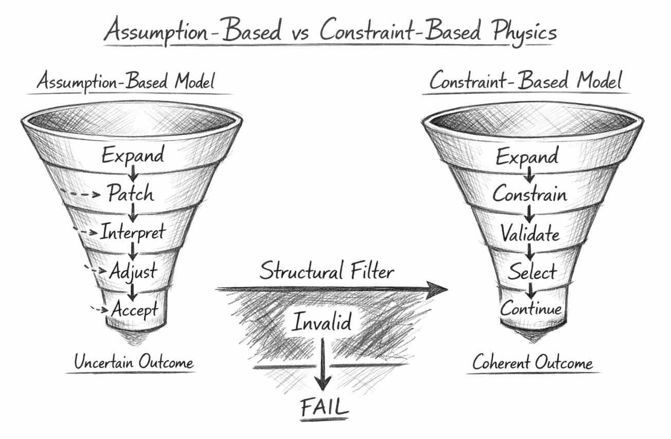
Expansion → Constraint → Survival Funnel

1. Overview

The diagram illustrates two fundamentally different structural approaches to physical theory:

  • Assumption-Based Physics (left funnel)
  • Constraint-Based Physics (right funnel)

Both begin with the same initial step:

\[ E = \operatorname{expand}(I, R) \]

However, they diverge in how they treat validity, constraint enforcement, and continuation.

2. The Left Funnel — Assumption-Based Expansion

The left-hand funnel represents the traditional modelling paradigm:

Flow Sequence

Expand→Patch→Interpret→Adjust→Accept


Scientific Interpretation

The theory generates candidate states using:

1. Expand

\[ O = f(I, \theta) \]

2. Patch

Divergences or inconsistencies are corrected through:

  • renormalisation,
  • parameter tuning,
  • auxiliary insertions.
3. Interpret

Multiple interpretations are introduced to reconcile results.

4. Adjust

Parameters or frameworks are modified to match observations.

5.Accept

A result is accepted based on:

  • empirical fit,
  • not structural necessity.

Key Property

\[ x \in E \;\not\Rightarrow\; x \models (B \land K) \]

Validity is not guaranteed—it is imposed after generation.


Outcome

Uncertain Outcome

The system:

  • may succeed empirically,
  • but lacks structural determinism and internal validity enforcement.

3. The Right Funnel — Constraint-Based Filtering

The right-hand funnel represents the constraint-based formulation introduced in this work.

Flow Sequence

Expand→Constrain→Validate→Select→Continue


Scientific Interpretation
1. Expand

As before:

\[ E = \operatorname{expand}(I, R) \]

2. Constrain

Boundary conditions and invariants are applied:

\[ (B, K) \]

3. Validate

Construct the admissible set:

\[ V = \{ x \in E \mid x \models (B \land K) \} \]

4. Select

A valid state is chosen:

\[ x^* \in V \]

5. Continue

Evolution proceeds only if:

\[ |V| > 0 \]


Key Property

\[ x \in E \;\Rightarrow\; x \text{ is accepted } \iff x \models (B \land K) \]

Validity is intrinsic, not imposed.


Outcome
Coherent Outcome

The system:

  • guarantees admissibility,
  • ensures structural consistency,
  • and defines continuation formally.

4. The Structural Filter — Failure Boundary

Between the funnels lies the structural filter, representing:

\[ V = \varnothing \]


Interpretation
  • All candidate states fail to satisfy constraints
  • No valid continuation exists

Formal Condition

\[ V = \varnothing \;\Rightarrow\; \text{FAIL} \]


Scientific Meaning

This replaces:

  • singularities,
  • divergences,
  • undefined behaviour

with a well-defined structural failure state.

5. Comparative Structural Insight

Property Assumption-Based Constraint-Based
Validity enforcement External Internal
Hidden assumptions (H) \(H \neq \emptyset\) \(H = \emptyset\)
Continuation Assumed Tested (\(V > 0\))
Failure definition Undefined Formal (\(V = \emptyset\))
Determinism Model-dependent Structure-dependent
Outcome type Approximate Coherent

6. Funnel Interpretation as State Compression

The funnel shape is not illustrative—it is mathematically meaningful:

  • The width represents the cardinality of state space
  • Narrowing represents constraint enforcement
Left Funnel

Reduction occurs via:

  • interpretation,
  • adjustment,
  • external correction
→ non-formal compression

Right Funnel

Reduction occurs via:

\[ E \to V \]

→ constraint-defined compression

7. Core Insight of the Diagram

The diagram encodes a single unifying statement:

\[ \text{Reality} \equiv \{ x \mid x \models (B \land K) \} \]


Implication
  • Physics is not about generating possibilities
  • It is about selecting valid states under constraint

8. Relation to Flow Algebra

This diagram is a direct visualisation of:

\[ \operatorname{Execution}(S) \equiv \operatorname{Select}\bigl(\operatorname{Validate}(\operatorname{Expand}(I, R))\bigr) \]

and its failure condition:

\[ V = \emptyset \Rightarrow \text{no coherent continuation} \]

9. Final Interpretation

The diagram formalises a shift:

From:

Generate → Repair → Interpret

To:

Generate → Constrain → Validate → Continue

This diagram demonstrates that coherence is not achieved by correcting outcomes, but by restricting existence to what satisfies constraint from the outset.

Diagram → Flow Mapping (Concise)

Diagram Stage Flow Algebra Representation Equation Form Scientific Meaning
Expand E := expand(I, R) $$E = \operatorname{expand}(I, R)$$ Generation of all candidate states permitted by the system rules
Patch external validity enforcement — Post-hoc correction (e.g. renormalisation, parameter tuning)
Interpret interpretive resolution — Multiple frameworks used to reconcile outputs
Adjust parameter/model modification — Model altered to match observations
Accept extrinsic acceptance — Output accepted without intrinsic validity guarantee
Invalid (Filter) V = ∅ ⇒ FAIL $$V = \emptyset \Rightarrow \text{FAIL}$$ No valid states satisfy constraints → no coherent continuation
Constrain apply (B, K) — Enforcement of boundary conditions and invariants
Validate V := {x ∈ E | x ⊨ (B ∧ K)} $$V = \{x \in E \mid x \models (B \land K)\}$$ Construction of the admissible state space
Select x* ∈ V $$x^* \in V$$ Selection of a valid state from the admissible set
Continue |V| > 0 $$|V| > 0$$ Continuation exists only if valid states are non-empty

The diagram maps directly to the flow by showing that constraint-based systems do not correct invalid states—they eliminate them from existence.

\[ \text{Reality} \equiv \{ x \mid x \models (B \land K) \} \]

Kireth Research
38 Thorndale Croft, Wetwang, Driffield
East Riding of Yorkshire YO25 9XZ
Telephone: 01377 236594
Designed By