Chapter 47
Wavefunction as Coherence Map

Within conventional quantum mechanics, the wavefunction, usually denoted by $\Psi$, is regarded as the fundamental mathematical object describing a quantum system. It evolves continuously according to the Schrödinger equation and contains all measurable information about the system. However, despite nearly a century of extraordinary predictive success, the physical meaning of the wavefunction remains one of the deepest unresolved questions in modern physics. Competing interpretations variously describe it as a probability amplitude, a state of knowledge, an element of reality, a computational tool, or a branch-generating object within a multiverse.

Holographic Space-Time (HST) proposes an alternative interpretation. Rather than treating the wavefunction as the primary physical entity, HST identifies it as a derived geometric representation of a deeper recursive coherence structure encoded within the holographic boundary.

In this framework, matter, energy, fields, and quantum states do not exist independently inside space. Instead, they emerge from recursive updates of boundary information. The wavefunction therefore does not describe an object moving through space but rather provides a map of how coherent boundary configurations may project into observable reality.

The wavefunction is therefore promoted from being a mysterious mathematical amplitude into something with direct geometric meaning: a coherence map of recursively stable boundary configurations.

The traditional interpretation of quantum mechanics separates evolution into two incompatible processes:

1. Continuous deterministic evolution

\[ i\hbar\frac{\partial\Psi}{\partial t}=\hat{H}\Psi \]

and

2. Instantaneous wavefunction collapse during measurement.

The transition between these two behaviours has never received a universally accepted physical explanation.

Questions naturally arise:

These questions collectively define the measurement problem.

HST removes the need for an actual physical collapse.

Instead, recursive boundary evolution continuously updates coherence until only one configuration remains globally stable under the boundary constraints.

Observation is therefore not a discontinuity but a recursive coherence selection process.

Instead of representing probabilities directly, HST interprets the wavefunction as a geometric landscape over the space of allowable recursive boundary configurations.

Each point in this landscape corresponds to a possible recursive coherence solution.

The amplitude

\[ \left|\Psi\right| \]

measures the degree of recursive stability rather than the existence of a physical particle.

Large amplitudes correspond to:

Small amplitudes correspond to:

Thus the wavefunction becomes a map of recursive structural stability.

The logical progression within HST is

\[ B_t\rightarrow\Gamma_Q\rightarrow Q_t\rightarrow\Psi_t \]

where

The wavefunction therefore appears only after recursive coherence has already been established.

It is not fundamental.

It is a projection of deeper recursive geometry.

Quantum systems appear to evolve continuously because recursive boundary updates occur at every recursive iteration.

Successive recursive states satisfy

\[ B_t\rightarrow B_{t+1} \]

with only infinitesimal coherence modifications.

Consequently

\[ \Psi_t\rightarrow\Psi_{t+1} \]

also changes smoothly.

Continuous Schrödinger evolution therefore emerges naturally from continuous recursive boundary evolution.

Born's Rule states

\[ P=\left|\Psi\right|^2 \]

Within HST this is no longer a fundamental axiom.

Instead,

\[ \left|\Psi\right|^2 \]

measures the relative stability of competing recursive boundary solutions.

Configurations with greater recursive coherence survive more recursive updates.

Configurations with poor coherence disappear rapidly.

Probability therefore reflects long-term recursive persistence.

Observation samples the stability distribution rather than generating probabilities from nothing.

Quantum superposition is traditionally written

\[ \Psi=\sum_i c_i\psi_i \]

HST interprets this as

multiple simultaneously admissible recursive coherence pathways.

Each component

\[ \psi_i \]

represents an allowed recursive geometric solution.

No paradox arises because all coexist only as potential recursive boundary configurations.

Physical observation occurs only when recursive coherence selects a unique globally stable configuration.

Measurement introduces new boundary information.

The boundary evolves according to

\[ B_t\rightarrow B_{t}' \]

which modifies the coherence landscape.

Many previously admissible recursive solutions become inconsistent with the updated constraints.

Only one configuration remains maximally coherent.

Selection therefore satisfies

\[ q^{*}=\operatorname*{arg\,max}_{q_i}\Omega(q_i) \]

where

\[ \Omega \]

represents recursive coherence.

Observation therefore corresponds to coherence optimisation rather than wavefunction collapse.

Interference patterns arise naturally because recursive coherence pathways combine geometrically.

Constructive interference corresponds to

aligned recursive coherence.

Destructive interference corresponds to

mutually incompatible recursive geometry.

The resulting interference pattern visualises the underlying coherence landscape encoded by the holographic boundary.

When particles interact they become embedded within a common recursive boundary structure.

Instead of carrying independent wavefunctions,

their coherence maps become coupled.

Both systems therefore reference the same recursive boundary information.

Measurement updates this shared boundary.

The correlated outcomes appear instantaneous because both particles were never independent recursive systems.

Their wavefunctions describe different projections of one larger coherence geometry.

Macroscopic systems contain enormous recursive redundancy.

Environmental interactions continually suppress unstable coherence pathways.

Only one overwhelmingly stable recursive solution survives.

The wavefunction therefore becomes sharply localised.

This naturally produces classical behaviour without requiring a special quantum-to-classical boundary.

Classical mechanics emerges simply as the limit of overwhelming recursive coherence stability.

Within HST the Schrödinger equation is interpreted as the continuous evolution of recursive coherence geometry.

Rather than describing a physical wave propagating through empty space, it governs how the holographic boundary continually updates coherent configurations.

The evolution equation therefore represents the dynamics of recursive stability across the admissible configuration manifold, while the observed wavefunction is the visible projection of that evolving coherence structure.

This interpretation preserves the predictive success of conventional quantum mechanics while providing a geometric origin for wavefunction evolution.

One of the central principles of Holographic Space-Time is that observable quantities are never the underlying reality itself but projections of recursive boundary dynamics.

The wavefunction belongs to this class of emergent observables.

It is not the boundary.

It is not the recursion.

It is not the coherence itself.

Instead, it is the mathematical shadow cast by recursive coherence geometry into the observable domain.

In this way, the wavefunction serves as an interface between hidden recursive boundary information and measurable physical phenomena.

Within Holographic Space-Time, the wavefunction is reinterpreted as a coherence map generated by recursive holographic boundary dynamics rather than as a fundamental physical entity. Quantum amplitudes quantify the relative stability of recursively admissible boundary configurations, while Born probabilities emerge from the persistence of coherent solutions under recursive evolution.

Superposition represents the coexistence of multiple stable coherence pathways, interference reflects their geometric interaction, and measurement corresponds to recursive optimisation that selects the maximally coherent configuration instead of invoking a physical collapse.

Continuous Schrödinger evolution arises naturally from successive boundary updates, and entanglement is understood as the manifestation of a shared recursive coherence structure encoded within the holographic boundary.

In this formulation, the wavefunction is an emergent projection of deeper coherence geometry, providing a unified physical interpretation of quantum evolution, probability, measurement, and classical emergence within the recursive framework of HST.

This Flow Algebra implements a complete recursive model of the quantum wavefunction within the Holographic Space-Time (HST) framework.

Rather than treating the wavefunction as a fundamental physical object or an abstract mathematical probability amplitude, the flow defines it as an emergent coherence map generated by recursive holographic boundary dynamics.

The implementation formalises the progression from boundary information to observable quantum behaviour through a sequence of deterministic recursive operations, replacing the traditional distinction between wavefunction evolution and wavefunction collapse with a unified process of coherence optimisation.

The flow begins with the holographic boundary state,

\[ B_t \]

which contains the complete recursive informational description of the physical system at recursion step $t$. This boundary is not merely a spatial surface but the primary information-bearing structure from which all observable physics emerges.

From this boundary, the flow constructs the quantum coherence geometry,

\[ \Gamma_Q=\operatorname{GenerateGeometry}(B_t) \]

which represents the network of recursively consistent relationships encoded within the boundary. Unlike conventional quantum mechanics, where the geometry of Hilbert space is assumed a priori, HST derives quantum geometry directly from boundary information.

This first stage establishes the geometric substrate upon which quantum states are subsequently defined.

Once the coherence geometry has been generated, the flow constructs the manifold of physically admissible quantum configurations,

\[ Q_t=\{\,q\mid q \models \Gamma_Q\,\} \]

Rather than assuming that every mathematically valid quantum state exists physically, the flow explicitly filters the state space according to recursive coherence constraints.

Only those configurations compatible with the holographic boundary survive.

This implementation therefore replaces unrestricted Hilbert-space enumeration with a recursively constrained configuration manifold.

The central operation of the flow is the construction of the wavefunction,

\[ \Psi_t=\operatorname{Map}(Q_t,\Gamma_Q) \]

This represents one of the most significant conceptual changes introduced by HST.

Instead of treating the wavefunction as the primitive description of reality, the flow constructs it as a projection of recursive coherence geometry.

The wavefunction therefore functions as an emergent coordinate system that maps the recursive stability of the underlying boundary into a mathematically observable representation.

Nothing physically "waves" through space.

Rather, the wavefunction visualises the distribution of stable recursive boundary configurations.

The flow next evaluates

\[ \rho_C=\left|\Psi_t\right|^2 \]

which is interpreted not as a fundamental probability density but as a coherence density.

Within the HST framework, this quantity measures the local stability of recursive boundary configurations.

Regions of high coherence density correspond to strongly supported recursive structures that persist through successive boundary updates.

Regions of low coherence density correspond to unstable recursive configurations that are unlikely to survive continued recursion.

The familiar Born probability therefore emerges as a measurable consequence of recursive stability rather than an independent postulate.

The flow then identifies the set of admissible quantum pathways,

\[ V_t=\{\,q_i\in Q_t\mid\Omega(q_i)\geq\Omega_{\min}\,\} \]

where

\[ \Omega(q_i) \]

is the recursive coherence score associated with each configuration.

This step introduces an explicit stability criterion absent from conventional quantum mechanics.

Configurations are retained only if they exceed a minimum coherence threshold.

The resulting set represents the physically meaningful quantum possibilities available to the system at the current recursive step.

If multiple admissible pathways remain,

\[ \left|V_t\right|>1 \]

the flow constructs the superposition

\[ \Psi_t=i\sum_i c_i q_i \]

Unlike conventional interpretations, this superposition is not regarded as multiple simultaneously existing physical realities.

Instead, each component represents a recursively stable coherence pathway encoded within the holographic boundary.

The coefficients

\[ c_i \]

measure the relative recursive stability of each pathway rather than the existence of parallel universes or indeterminate particles.

Superposition therefore becomes a geometric description of competing coherent solutions.

The flow explicitly enforces the condition

\[ i\sum_i P_t(q_i)=1 \]

where

\[ P_t(q_i)=\left|c_i\right|^2 \]

This ensures that the coherence map remains internally consistent.

Rather than viewing probability as an intrinsic property of microscopic systems, the flow interprets normalisation as the conservation of total recursive stability across the admissible configuration manifold.

Probability becomes a bookkeeping measure for recursive coherence.

Measurement is implemented through a modification of the holographic boundary,

\[ B_t'=\operatorname{UpdateBoundary}(B_t,M_t) \]

where

Mt​

represents the interaction introducing new boundary information.

This replaces the traditional concept of wavefunction collapse.

Instead of collapsing an abstract mathematical object, the boundary itself is updated.

The admissible configuration manifold is recalculated under the revised constraints,

\[ V_t'=\{\,q_i\in Q_t\mid q_i\models B_t'\,\} \]

causing previously admissible pathways to disappear naturally if they no longer satisfy the recursive coherence conditions.

Observation is therefore understood as recursive boundary refinement.

After updating the boundary, the flow selects the unique observed configuration by maximising recursive coherence,

\[ q^{*}=\operatorname*{arg\,max}_{q_i}\Omega(q_i) \]

This optimisation process replaces the postulated collapse mechanism of orthodox quantum mechanics.

The selected state is simply the configuration possessing the greatest global recursive consistency with the updated boundary information.

No discontinuous physical process is required.

The selected configuration is projected into the observable domain,

\[ O_t=\operatorname{Observe}(q^{*}) \]

where it becomes the experimentally measured quantum outcome.

Observation is therefore not an act that creates reality.

Instead, it is the visible manifestation of the most coherent recursive boundary solution.

The measured state represents the endpoint of recursive optimisation rather than an arbitrary probabilistic collapse.

The observed configuration is subsequently encoded back into the holographic boundary,

\[ B_{t+1}=\operatorname{Encode}(S_{t+1}) \]

completing the recursive cycle.

Every observation contributes new information to the boundary, altering the coherence landscape from which future wavefunctions are generated.

This recursive reintegration ensures that quantum evolution is a continuous feedback process rather than a sequence of disconnected measurements.

The flow explicitly implements constructive and destructive interference by comparing the recursive alignment of coherence pathways.

When pathways possess compatible recursive geometry, coherence increases, producing constructive interference.

When their recursive structures conflict, coherence decreases, producing destructive interference.

Interference therefore becomes a direct geometric consequence of boundary coherence rather than the mysterious interaction of probability amplitudes.

Entangled systems are implemented as quantum configurations sharing a common holographic boundary source.

Rather than exchanging information instantaneously across space, correlated systems reference the same recursive boundary information.

Measurement updates this shared boundary, and both subsystems remain consistent because they emerge from the same underlying coherence map.

This implementation removes the need for superluminal signalling while preserving the experimentally observed correlations.

The flow naturally reproduces the quantum-to-classical transition.

As environmental interactions recursively suppress unstable pathways, the admissible configuration set contracts,

\[ \left|V_t\right|\rightarrow 1 \]

Only one recursively stable solution remains.

The wavefunction therefore appears localised without requiring an additional collapse mechanism or special classical postulate.

Classical mechanics emerges simply as the limiting case of overwhelming recursive coherence.

The Flow Algebra presented in this chapter is a recursive computational description of how the quantum wavefunction emerges from holographic boundary coherence within the Holographic Space-Time (HST) framework.

Unlike conventional quantum mechanics, which begins by assuming the existence of a wavefunction and then prescribes its evolution using the Schrödinger equation, this flow derives the wavefunction from a deeper informational process.

The reader should therefore interpret the flow not as a sequence of mathematical manipulations, but as a chain of causal geometric transformations that progressively convert boundary information into observable quantum behaviour.

Each stage represents a well-defined recursive operation in which information is transformed while preserving coherence across the holographic boundary. Reading the flow correctly means following the evolution of boundary information as it is successively encoded, constrained, projected, optimised, observed, and finally reintegrated into the next recursive cycle.

The flow always begins with the holographic boundary state,

\[ B_t \]

which represents the complete recursive informational description of the system at recursion step $t$.

Within HST, this boundary is the primary physical entity.

It contains:

Nothing in the flow exists independently of this boundary.

The boundary should therefore be understood as the origin of every subsequent calculation.

The next operation,

\[ B_t\rightarrow\Gamma_Q \]

constructs the quantum coherence geometry.

This step should not be interpreted as creating physical particles or fields.

Instead, the recursive information stored on the boundary is organised into a geometric network describing every mutually consistent coherence relationship.

The geometry defines the structural rules governing which quantum configurations are physically admissible.

The reader should imagine this stage as constructing the geometric "landscape" upon which quantum behaviour can later emerge.

The coherence geometry immediately determines the manifold,

\[ Q_t \]

This manifold contains every recursively stable quantum configuration permitted by the boundary geometry.

Importantly,

not every mathematically imaginable state belongs to this manifold.

Only configurations satisfying the recursive coherence rules survive.

The flow therefore performs an automatic physical filtering process before any wavefunction is ever constructed.

The reader should recognise that HST generates quantum states from geometry rather than assuming an unrestricted Hilbert space.

The operation

\[ Q_t\rightarrow\Psi_t \]

is the conceptual centre of the chapter.

Here the recursive coherence geometry is projected into the familiar mathematical object known as the wavefunction.

The crucial point is that the wavefunction is not being created from nothing.

Instead, it is generated as a representation of the underlying coherence geometry.

When reading this stage, think of the wavefunction as a map.

Just as a geographical map represents a landscape without being the landscape itself, the wavefunction represents recursive coherence without being the underlying physical reality.

The projection translates hidden recursive geometry into a form that can be manipulated mathematically and compared with experimental observations.

Once the wavefunction exists, the flow computes

\[ \rho_C=\left|\Psi_t\right|^2 \]

Conventionally, this quantity is interpreted as a probability density.

Within HST it should instead be read as a coherence density.

Large values indicate regions of strong recursive stability.

Small values identify unstable or weakly supported recursive configurations.

When reading this stage, avoid thinking in terms of particles "having a higher probability of being somewhere."

Instead, interpret the density as measuring how strongly the boundary supports each recursive configuration.

Probability is an emergent consequence of stability rather than a fundamental property.

The flow next evaluates

\[ V_t=\{\,q_i\in Q_t\mid\Omega(q_i)\geq\Omega_{\min}\,\} \]

This operation removes every configuration whose recursive coherence falls below the required stability threshold.

Only physically meaningful pathways remain.

This stage should be understood as a recursive selection process.

The boundary continually eliminates incoherent possibilities while preserving stable ones.

The reader should view this as the mechanism through which physical reality naturally excludes unstable configurations.

If more than one admissible pathway survives,

\[ \left|V_t\right|>1 \]

the flow constructs

\[ \Psi_t=i\sum_i c_i q_i \]

In HST this does not imply that multiple physical universes coexist.

Instead, each component represents one recursively stable solution within the coherence landscape.

The coefficients

\[ c_i \]

measure the relative stability of these solutions.

The reader should therefore interpret superposition as the coexistence of multiple coherent possibilities encoded within the boundary, rather than multiple simultaneously realised realities.

The flow normalises

\[ P_t(q_i)=\left|c_i\right|^2 \]

ensuring

\[ \sum_i P_t(q_i)=1 \]

This stage conserves total recursive coherence.

The reader should understand probability as a stability weighting across competing recursive pathways.

Higher probabilities indicate configurations that possess greater recursive consistency with the holographic boundary.

This interpretation transforms Born's Rule from an independent axiom into a direct consequence of recursive coherence.

Measurement begins with

Mt​.

Rather than collapsing the wavefunction, the flow updates the boundary,

\[ B_t'=\operatorname{UpdateBoundary}(B_t,M_t) \]

This is one of the most important conceptual changes introduced by HST.

Nothing collapses.

Instead, new information modifies the recursive constraints governing admissible coherence.

The reader should visualise the coherence landscape itself changing shape.

Configurations that were previously stable may disappear, while others become favoured.

Measurement therefore corresponds to recursive geometric evolution rather than an instantaneous physical discontinuity.

After the boundary has been updated, the flow evaluates

\[ q^{*}=\operatorname*{arg\,max}_{q_i}\Omega(q_i) \]

This identifies the configuration possessing the highest recursive coherence.

The selected state is not chosen randomly.

Nor is it created during observation.

It already exists within the coherence landscape as the most globally consistent recursive solution.

The optimisation simply identifies it.

Readers should interpret this step as the recursive equivalent of finding the lowest-energy configuration in classical physics, except that optimisation occurs within coherence rather than energy.

Once the optimal configuration has been identified,

\[ O_t=\operatorname{Observe}(q^{*}) \]

produces the experimentally measurable outcome.

Observation does not generate physical reality.

It reveals the recursively selected configuration.

The observable world therefore represents the visible projection of recursive coherence optimisation.

Experimental measurements correspond to snapshots of this evolving recursive geometry.

The final stage,

\[ B_{t+1}=\operatorname{Encode}(S_{t+1}) \]

returns the observed state to the holographic boundary.

This completes one recursion.

Every observation modifies future boundary conditions.

Future wavefunctions therefore emerge from an updated informational landscape.

The reader should appreciate that the flow is circular rather than linear.

Every completed observation becomes part of the boundary from which future quantum behaviour is generated.

Reality continuously rewrites its own coherence map through recursive feedback.

Although the flow is presented as a sequence of discrete stages for clarity, it represents a continuously operating recursive process.

Each recursion step smoothly transforms boundary information into geometry, geometry into wavefunctions, wavefunctions into observable coherence densities, coherence densities into admissible pathways, and finally observed outcomes back into updated boundary information.

There is no abrupt transition between quantum evolution and measurement.

Instead, every stage is part of a single uninterrupted recursive cycle governed by coherence preservation.

This continuity explains why quantum systems exhibit smooth evolution between observations while still producing discrete measurement outcomes.

The central lesson when reading this flow is that the wavefunction is not the starting point of quantum physics.

It is the midpoint of a deeper recursive process.

The true causal sequence is:

Boundary→Geometry→Quantum Configurations→Wavefunction→Coherence Density→Stable Pathways→Measurement→Observation→Updated Boundary.

This reverses the conventional interpretation of quantum mechanics by placing holographic boundary information at the foundation of physical reality and treating the wavefunction as an emergent mathematical representation of recursive coherence.

This Flow Algebra should be read as a recursive execution model describing how holographic boundary information generates observable quantum phenomena. Each stage performs a specific geometric transformation: the boundary produces quantum coherence geometry, the geometry defines the admissible configuration manifold, the manifold is projected into the wavefunction, coherence density measures recursive stability,

stable pathways form quantum superpositions, measurement updates the boundary rather than collapsing the wavefunction, coherence optimisation selects the globally consistent configuration, and observation projects that configuration into measurable reality before reintegrating the result into the evolving holographic boundary.

The flow therefore provides a unified recursive interpretation of quantum mechanics in which wavefunctions, probabilities, interference, entanglement, and measurement all emerge naturally from the continuous evolution of boundary coherence, eliminating the conceptual divide between quantum evolution and observation while preserving the predictive structure of quantum theory.

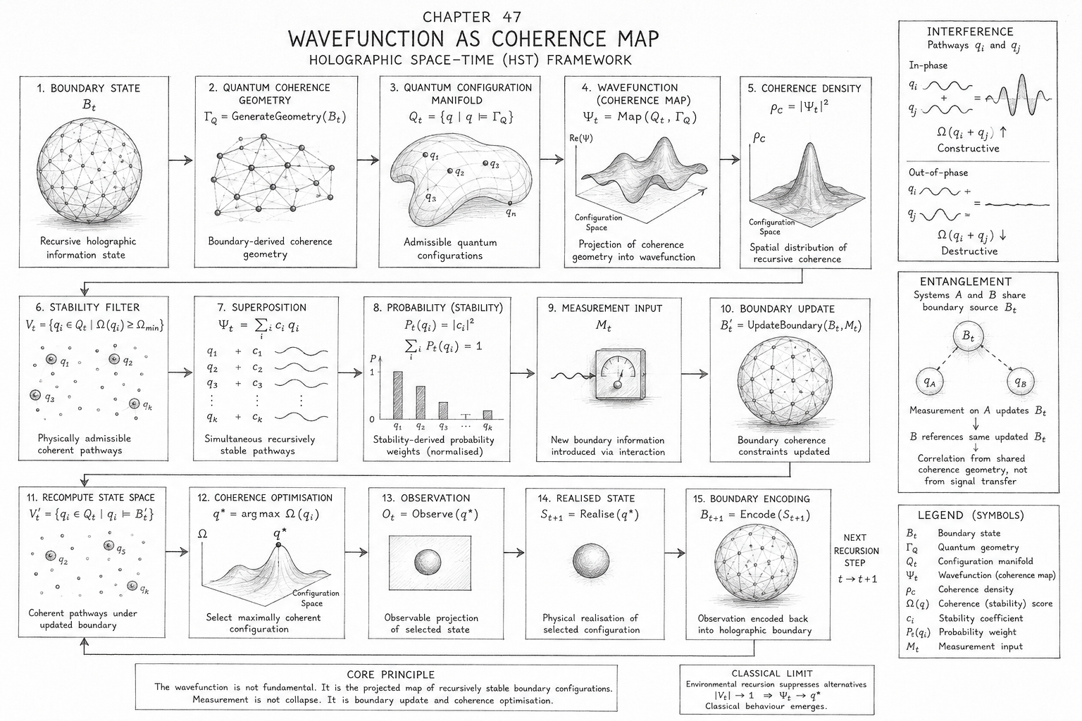
The scientific pencil diagram for Chapter 47 illustrates one of the central ideas of the Holographic Space-Time (HST) framework: the quantum wavefunction is not a fundamental physical entity but an emergent coherence map generated by recursive holographic boundary dynamics.

Rather than depicting particles existing within a pre-existing spatial arena, the illustration presents a continuous sequence of recursive transformations through which boundary information is converted into quantum observables.

Each panel represents a distinct stage in the recursive evolution of coherence, demonstrating how quantum states, probabilities, interference, measurement, and observation all arise naturally from the underlying boundary geometry.

The diagram is intentionally organised from left to right to emphasise causal progression. Unlike traditional quantum-mechanical diagrams that begin with a wavefunction, this illustration begins with the holographic boundary itself, reflecting the HST principle that information encoded on the recursive boundary precedes all observable physical phenomena.

The first panel presents the holographic boundary,

\[ B_t \]

as a recursively connected informational network.

Rather than representing a physical surface enclosing space, the spherical lattice symbolises the complete recursive information state of the system at recursion step $t$. Every node corresponds to locally encoded information, while every connecting edge represents recursive coherence relationships linking neighbouring regions of the boundary.

This panel establishes the fundamental assumption of HST: the boundary is the primary physical object, and everything that follows is derived from its recursive informational content. No particles, fields, or wavefunctions exist independently of this structure.

The second panel transforms the boundary into the quantum coherence geometry,

\[ \Gamma_Q=\operatorname{GenerateGeometry}(B_t) \]

The interconnected graph illustrates how recursive boundary information is organised into a network of mutually consistent coherence relationships. Unlike the boundary, which stores information, the geometry expresses the structural rules governing how that information can evolve while maintaining recursive consistency.

This panel demonstrates that quantum geometry is generated rather than assumed. In HST, geometry is not imposed externally but emerges directly from recursive boundary organisation.

The third panel depicts the admissible quantum configuration manifold,

\[ Q_t=\{\,q\mid q\models\Gamma_Q\,\} \]

The smoothly contoured surface represents the complete set of recursively admissible quantum configurations. Individual points labelled $q_1$, $q_2$, $q_3$, and $q_n$ correspond to candidate coherence pathways permitted by the underlying geometry.

The irregular boundary of the manifold is significant. It illustrates that recursive coherence imposes natural constraints on the available state space. Only configurations satisfying the boundary-derived coherence geometry are retained, while incoherent solutions are excluded before the wavefunction is even constructed.

The fourth panel is the conceptual centre of the chapter.

Here the flow generates the wavefunction,

\[ \Psi_t=\operatorname{Map}(Q_t,\Gamma_Q) \]

The three-dimensional undulating surface is deliberately drawn as a topographic landscape rather than as a physical wave travelling through space. Peaks represent highly coherent recursive configurations, valleys correspond to weakly supported configurations, and the overall surface visualises the recursive stability landscape encoded by the holographic boundary.

The illustration reinforces one of HST's central claims: the wavefunction is a map of coherence, not a physical substance. Just as a geographical map represents terrain without being the terrain itself, the wavefunction represents recursive boundary structure without constituting the underlying reality.

The fifth panel evaluates

\[ \rho_C=\left|\Psi_t\right|^2 \]

The pronounced central peak illustrates a region of maximum recursive coherence. Rather than representing the location of a particle, the peak signifies the region where the holographic boundary most strongly supports a recursively stable configuration.

The vertical axis labelled $\rho_C$ measures coherence density, while the horizontal plane represents configuration space. This visualisation replaces the conventional probability-density interpretation with one based on recursive structural stability.

The sixth panel introduces the recursive filtering process,

\[ V_t=\{\,q_i\in Q_t\mid\Omega(q_i)\geq\Omega_{\min}\,\} \]

Only a subset of the initially available configurations remains highlighted. These surviving nodes correspond to quantum pathways possessing sufficient recursive coherence to remain physically admissible.

The faded background points represent unstable configurations that fail the coherence threshold and are therefore excluded from further evolution. This panel demonstrates that HST performs a deterministic stability selection before measurement occurs.

The seventh panel illustrates

\[ \Psi_t=i\sum_i c_i q_i \]

Each candidate pathway is paired with its stability coefficient,

\[ c_i \]

The parallel waveforms do not represent simultaneously existing particles. Instead, they visualise multiple recursively stable coherence pathways coexisting within the holographic boundary.

Superposition is therefore interpreted as a structured coherence landscape rather than a literal coexistence of mutually exclusive physical realities.

The eighth panel displays

\[ P_t(q_i)=\left|c_i\right|^2 \]

together with the normalisation condition,

\[ \sum_i P_t(q_i)=1 \]

The histogram illustrates the relative recursive stability of the remaining coherence pathways. Taller bars correspond to configurations possessing greater recursive support from the holographic boundary.

Probability is therefore interpreted as a measurable expression of recursive stability rather than as an intrinsic property of microscopic objects.

The ninth panel introduces the measurement interaction,

\[ M_t \]

The instrument symbol represents any physical interaction capable of introducing new information into the recursive boundary.

The incoming wave signifies information entering the holographic system rather than an external observer collapsing a wavefunction. Measurement is therefore redefined as boundary information acquisition.

The tenth panel shows

\[ B_t'=\operatorname{UpdateBoundary}(B_t,M_t) \]

The boundary network appears subtly rearranged, reflecting the modification of recursive coherence constraints following measurement.

This panel replaces the conventional concept of wavefunction collapse with recursive boundary evolution. The geometry itself changes, naturally altering the set of admissible coherence pathways.

Following the boundary update, the admissible configuration manifold is recalculated,

\[ V_t'=\{\,q_i\in Q_t\mid q_i\models B_t'\,\} \]

Several previously admissible configurations have disappeared. The remaining pathways are those compatible with the updated coherence geometry.

This stage demonstrates that quantum measurement is fundamentally a process of constraint refinement, not probabilistic collapse.

The twelfth panel performs the optimisation,

\[ q^{*}=\operatorname*{arg\,max}_{q_i}\Omega(q_i) \]

The central peak identifies the unique recursively optimal configuration. Rather than selecting an outcome randomly, the recursive system identifies the configuration possessing maximum global coherence.

This optimisation is entirely deterministic within the recursive framework.

The thirteenth panel projects the selected configuration into observable reality,

\[ O_t=\operatorname{Observe}(q^{*}) \]

The isolated sphere symbolises the experimentally measurable quantum state.

Importantly, the observation does not create the state. It reveals the configuration previously selected through recursive coherence optimisation.

The realised state,

\[ S_{t+1}=\operatorname{Realise}(q^{*}) \]

represents the physical manifestation of the selected recursive configuration.

At this stage the optimisation process has completed, and the quantum system has entered its observable classical description.

The distinction between quantum possibility and realised observation disappears because only the maximally coherent configuration remains.

The final panel closes the recursive cycle through

\[ B_{t+1}=\operatorname{Encode}(S_{t+1}) \]

The observed state is written back into the holographic boundary, ensuring that future recursive evolution incorporates the newly acquired information.

This feedback process illustrates one of the defining characteristics of HST: every observation modifies the informational boundary from which future wavefunctions are generated, creating a continuously self-updating recursive universe.

The interference panel compares two coherence pathways,

\[ q_i,\;q_j \]

The upper illustration shows phase-aligned pathways producing constructive interference,

\[ \Omega(q_i+q_j)\uparrow \]

while the lower illustration depicts phase-opposed pathways producing destructive interference,

\[ \Omega(q_i+q_j)\downarrow \]

Rather than interpreting interference as the interaction of probability amplitudes in empty space, the diagram identifies it as the geometric addition or cancellation of recursive coherence within the holographic boundary.

The entanglement diagram illustrates two quantum systems,

\[ q_A,\;q_B \]

sharing a common boundary source,

\[ B_t \]

The diagram emphasises that both systems reference the same recursive coherence geometry. A measurement affecting one subsystem updates the shared boundary, automatically preserving consistency in the correlated subsystem.

No information propagates through space between the particles. Instead, both emerge from the same underlying coherence map.

The Wavefunction as Coherence Map Flow Algebra executes deterministically provided that a valid recursive holographic boundary state exists. Beginning with the boundary information state $B_t$, the flow generates the quantum coherence geometry $\Gamma_Q$, constructs the admissible quantum configuration manifold $Q_t$, projects that manifold into the emergent wavefunction $\Psi_t$, computes the recursive coherence density $\rho_C$, filters physically admissible coherence pathways $V_t$, constructs superposition through recursively stable pathway combinations, evaluates stability-derived probabilities, incorporates measurement as a recursive boundary update, recomputes the admissible state space, selects the globally maximally coherent configuration, projects that configuration into observable reality, realises the physical state, and recursively encodes the observation back into the holographic boundary for the next evolution cycle.

Execution is guaranteed whenever the recursive coherence constraints remain internally consistent.

Execution begins only if the holographic boundary satisfies

\[ B_t\neq\varnothing \]

The boundary must contain sufficient recursive information to generate a valid quantum coherence geometry.

If no boundary information exists,

\[ B_t=\varnothing \]

execution terminates immediately because no recursive quantum geometry can be constructed.

The recursive geometry generation stage guarantees

\[ \Gamma_Q=\operatorname{GenerateGeometry}(B_t) \]

Every admissible coherence relationship is derived directly from the holographic boundary.

No external geometry, hidden variables, or independently existing quantum state space is required.

The quantum geometry is therefore uniquely determined by the recursive informational content of the boundary.

The admissible quantum manifold satisfies

\[ Q_t=\{\,q\mid q\models\Gamma_Q\,\} \]

Every configuration within the manifold is guaranteed to satisfy the recursive coherence constraints generated by the boundary.

Configurations violating those constraints are excluded automatically.

No physically inconsistent quantum states can propagate through the remainder of the flow.

The wavefunction is guaranteed to be generated only from recursively admissible configurations,

\[ \Psi_t=\operatorname{Map}(Q_t,\Gamma_Q) \]

This guarantees that the wavefunction is always an emergent coherence map.

It is never treated as an independent physical object.

Every feature of the wavefunction corresponds directly to an underlying recursive boundary structure.

The recursive coherence density is uniquely determined by

\[ \rho_C=\left|\Psi_t\right|^2 \]

Within HST this quantity always measures recursive coherence rather than intrinsic probability.

Consequently, the computed density always represents the stability distribution of admissible recursive boundary configurations.

The admissible pathway set satisfies$${}_{}$$

\[ V_t=\{\,q_i\in Q_t\mid\Omega(q_i)\geq\Omega_{\min}\,\} \]

Every surviving pathway is guaranteed to exceed the minimum recursive coherence threshold.

Unstable recursive configurations cannot propagate into subsequent execution stages.

Whenever

\[ \left|V_t\right|>1 \]

the flow constructs

\[ \Psi_t=i\sum_i c_i q_i \]

Each component of the superposition is guaranteed to correspond to a recursively stable coherence pathway.

The coefficients

\[ c_i \]

represent recursive stability weightings only.

They never imply the existence of multiple simultaneously realised physical universes.

Recursive probability is always evaluated through

\[ P_t(q_i)=\left|c_i\right|^2 \]

subject to

\[ i\sum_i P_t(q_i)=1 \]

Normalisation guarantees conservation of total recursive coherence weighting across all admissible pathways.

No probability leakage or incoherent weighting can occur.

Measurement executes by updating the holographic boundary,

\[ B_t'=\operatorname{UpdateBoundary}(B_t,M_t) \]

The flow guarantees that measurement modifies recursive boundary constraints rather than collapsing the wavefunction.

Every observation therefore corresponds to deterministic recursive boundary evolution.

No discontinuous collapse operation is required.

Following measurement,

\[ V_t'=\{\,q_i\in Q_t\mid q_i\models B_t'\,\} \]

The updated configuration manifold is guaranteed to contain only pathways compatible with the revised boundary constraints.

Previously admissible configurations that become inconsistent are removed automatically.

State selection is guaranteed through

\[ q^{*}=\operatorname*{arg\,max}_{q_i}\Omega(q_i) \]

The selected configuration always possesses the greatest recursive coherence among all admissible pathways.

Selection therefore results from deterministic optimisation rather than stochastic collapse.

Observation executes through

\[ O_t=\operatorname{Observe}(q^{*}) \]

The observable state is guaranteed to be the projection of the recursively optimal configuration.

Observation never creates physical reality.

It reveals the already selected maximally coherent recursive solution.

The realised state satisfies

\[ S_{t+1}=\operatorname{Realise}(q^{*}) \]

which is recursively encoded as

\[ B_{t+1}=\operatorname{Encode}(S_{t+1}) \]

Every observation therefore contributes directly to the recursive evolution of the holographic boundary.

Information is preserved across recursion, ensuring continuous self-consistent system evolution.

The flow guarantees preservation of the following invariants throughout execution:

Boundary existence:

\[ B_t\neq\varnothing \]

Geometry consistency:

\[ \Gamma_Q=\operatorname{GenerateGeometry}(B_t) \]

Admissible state existence:

\[ V_t\neq\varnothing \]

Probability conservation:

\[ \sum_i P_t(q_i)=1 \]

Coherence maximisation:

\[ q^{*}=\operatorname*{arg\,max}_{q_i}\Omega(q_i) \]

Recursive information continuity:

\[ B_t\rightarrow B_{t+1} \]

These invariants guarantee that recursive coherence is preserved throughout every execution cycle.

Execution terminates only if one or more of the following conditions occur:

\[ B_t=\varnothing \]

No holographic boundary information exists.

\[ \Gamma_Q=\varnothing \]

Recursive coherence geometry cannot be generated.

\[ Q_t=\varnothing \]

No admissible quantum configurations satisfy the generated geometry.

\[ V_t=\varnothing \]

No recursively stable pathways exceed the coherence threshold.

\[ i\sum_i P_t(q_i)\neq 1 \]

Probability normalisation is violated.

\[ \Omega(q^{*})<\Omega_{\min} \]

No configuration satisfies the minimum recursive coherence required for observation.

If none of these conditions occur, execution proceeds deterministically to completion.

This execution is guaranteed to produce a mathematically consistent and recursively deterministic implementation of Wavefunction as Coherence Map within the Holographic Space-Time framework.

The flow guarantees that the wavefunction is always generated as an emergent projection of recursive boundary coherence, that probabilities arise from recursive stability rather than fundamental randomness, that measurement is implemented through recursive boundary refinement instead of wavefunction collapse, and that every observation is encoded back into the holographic boundary to preserve continuous recursive evolution.

Consequently, the complete quantum measurement cycle is executed as a single self-consistent recursive process in which geometry, coherence, observation, and evolution remain unified under the holographic boundary formalism.