Chapter 16
Constraint Propagation

Constraint Preservation
Author: Mark Higgins
© Mark Anthony Higgins 11 October 2025
Revised Date: 08 May 2026
Audio Overview

Introduction

Constraint propagation is the recursive distribution of structural requirements across a dynamic system in order to preserve admissibility, coherence, and stable continuation. Within classical computation, constraint propagation is commonly used in logic solving, optimization systems, symbolic reasoning, and state validation. In Flow Algebra, however, constraint propagation is not merely a computational technique — it is a foundational mechanism governing how recursive systems preserve structural existence.

A recursive system cannot evolve arbitrarily. Every future state must satisfy a collection of admissibility conditions that define whether continuation remains structurally valid. These conditions propagate through the system recursively, constraining possible future trajectories and eliminating incompatible state transitions.

Constraint propagation therefore defines the geometry of survivable evolution.

Recursive State Structure

Flow Algebra represents a recursive system as:

\[ S_t = (I_t, R, B, K) \]

Where:

  • ItI_t = informational state at time tt
  • RR = recursive transformation rules
  • BB = boundary constraints
  • KK = invariant-preservation conditions

The system evolves by generating candidate future states:

\[ E_t = \operatorname{expand}(I_t, R) \]

However, not all generated states are admissible. Constraint propagation recursively filters invalid continuations from the candidate state space.

Admissibility Filtering

Constraint propagation operates through recursive admissibility filtering:

\[ V_t = \{x \in E_t \mid x \models (B \land K)\} \]

Where:

  • EtE_t = expanded candidate state space
  • VtV_t = admissible continuation set
  • x⊨(B∧K)x \models (B \land K) indicates that state xx satisfies all boundary and invariant requirements

Only structurally admissible states survive recursive continuation.

This transforms computation from unrestricted generation into constrained survivability selection.

Constraint Propagation as Structural Survival

In Flow Algebra, constraints are not external restrictions arbitrarily imposed on a system. Constraints define the structural conditions required for recursive persistence itself.

A valid state is therefore not merely “allowed.”

A valid state is structurally survivable.

Constraint propagation recursively distributes these survivability conditions throughout the system, ensuring that incompatible trajectories are eliminated before recursive instability spreads.

This yields a deeper interpretation of recursive execution:

Existence≡Admissible Recursive Continuation

A system exists recursively only while admissible future states remain available.

Recursive Collapse Conditions

If constraint propagation eliminates all admissible future states, recursive continuation fails:

\[ V_t = \varnothing \;\Rightarrow\; \mathrm{FAIL} \]

This represents recursive collapse.

The collapse condition emerges not because the system “chooses” termination, but because no structurally coherent continuation remains compatible with the propagated constraints.

Constraint propagation therefore governs both:

  • recursive survival,
  • and recursive termination.

Local Constraints and Global Coherence

Constraint propagation transforms local conditions into global system behavior.

A contradiction introduced in one region of a recursive system propagates through dependency relationships into surrounding structures. The larger and more interconnected the recursive system becomes, the more important propagation stability becomes for preserving global coherence.

Thus:

  • local inconsistency produces propagated structural tension,
  • propagated tension reduces admissible continuation space,
  • reduced continuation space increases collapse probability.

Constraint propagation therefore acts as the stabilizing mechanism linking local state validity to global recursive integrity.

Constraint Propagation in Computation

Within computational systems, constraint propagation appears in:

  • logic solvers,
  • symbolic theorem systems,
  • recursive optimization,
  • type systems,
  • state validation architectures,
  • dependency resolution engines,
  • recursive AI reasoning systems.

Flow Algebra generalizes these isolated computational mechanisms into a unified recursive framework.

Computation becomes:

Computation≡Recursive Constraint Stabilization

A computation succeeds only if admissible recursive continuation remains structurally available throughout execution.

Constraint Propagation in Physics

Within physical systems, constraint propagation manifests as coherence-preserving field evolution.

Examples include:

  • conservation laws,
  • causal consistency,
  • relativistic invariants,
  • quantum admissibility conditions,
  • field continuity requirements,
  • entropy constraints.

Physical reality itself may therefore be interpreted as a recursively constrained admissibility structure.

Stable physical systems survive because invalid configurations are recursively eliminated through propagated coherence restrictions.

This reframes physics from force interaction alone into recursive coherence management across constrained state geometry.

Constraint Propagation in Cognition and AI

In recursive cognition systems, constraint propagation governs reasoning stability.

Thought processes generate candidate inference states:

\[ E_t = \operatorname{expand}(I_t, R) \]

Recursive coherence filtering then removes contradictory or unstable reasoning paths:

\[ V_t = \{x \in E_t \mid x \models (B \land K)\} \]

Contradictions propagate recursively through inference networks until one of three outcomes occurs:

  • 1. coherence restoration,
  • 2. boundary adaptation,
  • 3. recursive collapse.

Intelligence therefore emerges as the ability to maintain stable recursive propagation under increasing structural complexity.

Constraint Propagation as Recursive Geometry

Constraint propagation defines the geometry of recursive evolution.

The system does not traverse arbitrary possibility space.

It traverses only structurally admissible continuation space.

This transforms recursion into a constrained geometric flow through survivable state topology.

Future evolution becomes shaped not by arbitrary generation, but by recursively propagated admissibility structure.

Structural Implications

Constraint propagation produces several foundational consequences:

  • Recursive systems survive only through admissible continuation.
  • Local contradictions generate global recursive effects.
  • Stable intelligence requires propagation management.
  • Physics preserves coherence through propagated invariants.
  • Computation is fundamentally constraint filtering.
  • Reality evolves through recursive admissibility geometry.

Constraint propagation therefore serves as one of the foundational mechanisms underlying recursive coherence systems.

Chapter Summary

Constraint propagation is the recursive distribution of admissibility conditions across dynamic systems. In Flow Algebra, it governs how systems preserve coherence, eliminate contradictions, and maintain recursive continuity.

The system evolves by:

  • 1. generating candidate continuations,
  • 2. propagating structural constraints,
  • 3. filtering invalid states,
  • 4. preserving admissible recursive trajectories.

Formally:

\[ E_t = \operatorname{expand}(I_t, R) \]

\[ V_t = \{x \in E_t \mid x \models (B \land K)\} \]

\[ V_t = \varnothing \;\Rightarrow\; \mathrm{FAIL} \]

Constraint propagation therefore defines the mechanism through which recursive systems preserve structural survival across time, computation, cognition, and physical reality.

flow "ConstraintPropagation" v1.0

purpose:
  define: "Constraint propagation as recursive distribution of admissibility conditions across candidate state space."
  claim: "A recursive system continues only when at least one generated future state satisfies propagated boundary and invariant constraints."

state:
  S_t:
    structure: "(I_t, R, B, K)"
    I_t: "current information state"
    R: "recursive transformation rules"
    B: "boundary constraints"
    K: "invariant preservation conditions"

expand:
  input: I_t
  rule: R
  output: E_t
  equation: "E_t = expand(I_t, R)"
  meaning: "Generate possible recursive continuations from the current state."

propagate_constraints:
  across: E_t
  constraints:
    - B
    - K
  equation: "x ⊨ (B ∧ K)"
  meaning: "Each candidate continuation is tested against propagated boundary and invariant requirements."

filter:
  input: E_t
  condition: "x ⊨ (B ∧ K)"
  output: V_t
  equation: "V_t = { x ∈ E_t | x ⊨ (B ∧ K) }"
  meaning: "Only structurally admissible continuations survive."

select:
  from: V_t
  condition: "V_t ≠ ∅"
  output: x_star
  deterministic:
    when: "|V_t| = 1"
    equation: "x* ∈ V_t"
  probabilistic:
    when: "|V_t| > 1"
    equation: "x* = argmax_{x ∈ V_t} P(x | I_t, R, B, K)"
  meaning: "Select the surviving continuation with highest structural coherence."

update:
  input:
    - I_t
    - x_star
  output: I_t+1
  equation: "I_{t+1} = update(I_t, x*)"
  guarantee: "I_{t+1} ⊨ (B ∧ K)"
  meaning: "The system advances only through a constraint-valid continuation."

collapse:
  condition: "V_t = ∅"
  output: FAIL
  equation: "V_t = ∅ ⇒ FAIL"
  meaning: "If no candidate satisfies propagated constraints, recursive continuation terminates."

execution:
  condition: "V_t ≠ ∅"
  equation: "Execution(S_t) ⇔ V_t ≠ ∅"
  meaning: "Execution is equivalent to the existence of at least one admissible recursive continuation."

invariants:
  admissibility:
    equation: "∀x ∈ V_t, x ⊨ B"
  coherence:
    equation: "∀x ∈ V_t, x ⊨ K"
  continuation:
    equation: "I_{t+1} ⊨ (B ∧ K)"
  fixed_structure:
    equation: "(I_t, R, B, K) fixed ⇒ V_t fixed"

monitors:
  empty_valid_set:
    watch: "V_t = ∅"
    response: "terminate recursive execution"
  boundary_violation:
    watch: "∃x ∈ E_t : x ⊭ B"
    response: "remove x from admissible continuation set"
  invariant_violation:
    watch: "∃x ∈ E_t : x ⊭ K"
    response: "remove x from admissible continuation set"
  propagation_failure:
    watch: "constraints fail to propagate across dependent regions"
    response: "mark system as structurally unstable"

output:
  success:
    condition: "V_t ≠ ∅"
    result: "S_{t+1}"
    equation: "S_t → E_t → V_t → x* → S_{t+1}"
  failure:
    condition: "V_t = ∅"
    result: "FAIL"

summary:
  statement: "Constraint propagation ensures that recursive systems evolve only through states that satisfy propagated boundary and invariant conditions."

What This Flow Implements

Constraint Propagation

The Constraint Propagation flow implements a recursive admissibility system in which structural requirements distribute across candidate state space in order to preserve coherent continuation. Rather than allowing unrestricted recursive evolution, the system continuously propagates boundary and invariant constraints throughout all possible future states, eliminating structurally invalid continuations before execution proceeds.

At its core, the flow defines recursion as a constrained survivability process.

The system begins with a recursive state structure:

\[ S_t = (I_t, R, B, K) \]

where:

  • ItI_t represents the current informational configuration,
  • RR defines recursive transformation rules,
  • BB defines boundary constraints,
  • KK defines invariant-preservation conditions.

The flow first generates an expanded candidate continuation space:

\[ E_t = \operatorname{expand}(I_t, R) \]

This expansion represents all structurally reachable future states prior to admissibility filtering.

The central mechanism implemented by the flow is recursive constraint propagation:

\[ V_t = \{x \in E_t \mid x \models (B \land K)\} \]

Every candidate state is recursively tested against propagated structural requirements. Only states satisfying all boundary and invariant conditions survive into the admissible continuation set VtV_t.

The flow therefore implements:

  • recursive admissibility filtering,
  • distributed structural validation,
  • contradiction elimination,
  • invariant preservation,
  • recursive survivability enforcement,
  • coherence-preserving continuation selection.

The system does not compute arbitrary futures.

It computes only structurally survivable continuations.

The flow additionally implements recursive collapse detection:

\[ V_t = \varnothing \;\Rightarrow\; \mathrm{FAIL} \]

If propagated constraints eliminate all candidate states, recursive continuation becomes impossible and execution terminates. This establishes recursive existence as dependent upon admissible continuation availability.

The flow also implements recursive continuation selection:

\[ x^* = \operatorname*{arg\,max}_{x \in V_t} P(x \mid I_t, R, B, K) \]

This allows the system to select the most structurally coherent continuation among all admissible candidates.

Once selected, the recursive state updates according to:

\[ I_{t+1} = \operatorname{update}(I_t, x^*) \]

while preserving propagated coherence:

\[ I_{t+1} \models (B \land K) \]

The flow therefore guarantees that successful recursive continuation preserves structural validity across state evolution.

Structural Behaviors Implemented

The flow implements several fundamental recursive behaviors:

1. Recursive Constraint Distribution

Constraints propagate throughout the entire candidate state space rather than remaining localized. Structural requirements recursively influence all dependent continuations.


2. Admissibility Filtering

Invalid continuations are removed before recursive execution advances. The system therefore evolves only through structurally coherent pathways.


3. Contradiction Elimination

Candidate states violating propagated constraints are recursively excluded from admissible continuation space.


4. Invariant Preservation

Core structural identities remain preserved throughout recursive evolution:

\[ \forall x \in V_t,\; x \models K \]


5. Boundary Enforcement

All surviving continuations satisfy recursive boundary conditions:

\[ \forall x \in V_t,\; x \models B \]


6. Recursive Survival Enforcement

The existence of recursive continuation depends entirely on the survival of admissible future states:

\[ \mathrm{Execution}(S_t) \;\Longleftrightarrow\; V_t \neq \varnothing \]


7. Recursive Collapse Detection

If no admissible continuation survives propagation filtering, recursive execution terminates automatically.


Computational Meaning

Within computation, this flow implements:

  • recursive validation systems,
  • symbolic constraint solvers,
  • dependency propagation systems,
  • admissibility filtering architectures,
  • recursive theorem validation,
  • type consistency enforcement,
  • probabilistic reasoning stabilization,
  • AI contradiction filtering.

The flow reframes computation as recursive coherence stabilization rather than unrestricted symbolic manipulation.


Physical Interpretation

Within physical systems, the flow implements:

  • conservation enforcement,
  • coherence-preserving field evolution,
  • admissible state stabilization,
  • causal consistency propagation,
  • entropy boundary regulation,
  • quantum state admissibility filtering.

Physical reality itself becomes interpretable as recursively propagated structural admissibility.

Cognitive Interpretation

Within cognition and AI, the flow implements:

  • recursive contradiction management,
  • stable inference propagation,
  • coherence-preserving reasoning,
  • belief consistency filtering,
  • recursive self-stabilization,
  • structural reasoning continuity.

Intelligence becomes the ability to maintain recursive admissibility under expanding structural complexity.

Foundational Principle Implemented

The deepest principle implemented by this flow is:

Existence≡Admissible Recursive Continuation

A recursive system exists only while propagated constraints permit structurally coherent continuation.

Constraint propagation therefore serves as one of the foundational mechanisms governing recursion, computation, cognition, and coherent reality itself.

How to Read This Flow

Constraint Propagation

The Constraint Propagation flow describes how recursive systems preserve structural coherence by distributing admissibility conditions across all possible future states. The flow should not be interpreted as ordinary procedural code. Instead, it represents a recursive structural execution model governing how valid continuation emerges from constrained state evolution.

This flow is read as a recursive survivability pipeline.

The system continuously:

  • 1. generates candidate future states,
  • 2. propagates structural constraints,
  • 3. removes invalid continuations,
  • 4. selects coherent survivable states,
  • 5. advances recursive execution.

The flow therefore describes how coherent systems maintain existence through admissibility preservation.

1. Read the Recursive State Definition First

The flow begins with the recursive system definition:

\[ S_t = (I_t, R, B, K) \]

This equation defines the complete recursive state structure.

Each component has a specific structural role:

Component Meaning
\( I_t \) Current informational state
\( R \) Recursive transformation rules
\( B \) Boundary constraints
\( K \) Invariant-preservation conditions

This sequence defines recursive existence through propagated admissibility.

2. Read Expansion as Candidate Generation

The next stage defines recursive expansion:

\[ E_t = \operatorname{expand}(I_t, R) \]

This operation generates the candidate continuation space.

Importantly

  • EtE_t does not represent valid states,
  • it represents possible states.

The expansion stage intentionally over-generates continuations before structural filtering occurs.

You should therefore interpret EtE_t as a temporary recursive possibility field.

3. Read Constraint Propagation as Recursive Filtering

The core of the flow is the admissibility filter:

\[ V_t = \{x \in E_t \mid x \models (B \land K)\} \]

This equation is the central structural operation.

Read it carefully in stages:

Symbol Meaning
\( x \in E_t \) Candidate continuation
\( \models \) Structurally satisfies
\( B \) Boundary constraints
\( K \) Invariant requirements
\( B \land K \) Both conditions simultaneously
\( V_t \) Admissible continuation set

The equation states:

“Only candidate states satisfying all propagated structural constraints survive recursive continuation.”

This is the primary mechanism of constraint propagation.

The flow therefore does not compute by unrestricted generation.

It computes by recursive elimination of invalid structure.

4. Read Propagation as Distributed Structural Influence

Constraint propagation means that structural requirements recursively distribute across all dependent future states.

A local contradiction does not remain isolated.

Instead:

  • incompatibilities propagate,
  • admissible continuation space contracts,
  • recursive tension increases,
  • unstable pathways collapse.

You should therefore read the flow as a dynamic recursive filtering field rather than a linear instruction sequence.

The system continuously reshapes future state space through propagated coherence requirements.

5. Read Selection as Survivable Continuation Choice

Once admissible states survive filtering, the system selects a continuation:

\[ x^* = \operatorname*{arg\,max}_{x \in V_t} P(x \mid I_t, R, B, K) \]

This equation selects the highest-coherence continuation from the admissible set.

Read the equation structurally:

Component Meaning
\( V_t \) Surviving admissible states
\( P(x \mid \ldots) \) Structural continuation weighting
\( \arg\max \) Highest-validity selection
\( x^* \) Selected continuation

The system therefore evolves through the most structurally coherent survivable pathway available.

6. Read Update as Recursive Continuation

The recursive update stage is:

\[ I_{t+1} = \operatorname{update}(I_t, x^*) \]

This operation advances the recursive state forward.

Importantly:

\[ I_{t+1} \models (B \land K) \]

The updated state preserves all propagated structural requirements.

The flow therefore guarantees recursive coherence preservation during successful execution.

7. Read Collapse as Structural Non-Existence

One of the most important equations in the flow is:

\[ V_t = \varnothing \;\Rightarrow\; \mathrm{FAIL} \]

This defines recursive collapse.

Read this literally:

  • no admissible states survive,
  • no valid continuation exists,
  • recursive execution terminates.

This is not merely an error condition.

It represents structural non-survivability.

The flow therefore defines existence itself as dependent upon admissible recursive continuation.

8. Read Execution as Admissible Continuation

The execution condition is:

\[ \mathrm{Execution}(S_t) \;\Longleftrightarrow\; V_t \neq \varnothing \]

This equation should be interpreted as:

“A recursive system continues existing only while at least one admissible continuation survives propagated constraints.”

Execution is therefore equivalent to recursive survivability.

9. Read the Flow as Recursive Geometry

This flow should ultimately be interpreted geometrically.

The recursive system moves through:

  • possibility space,
  • admissibility topology,
  • coherence boundaries,
  • invariant-preserving pathways.

Constraint propagation shapes the geometry of survivable future evolution.

The system does not move freely through arbitrary state space.

It moves only through recursively admissible continuation regions.

10. Structural Interpretation of the Entire Flow

The full recursive structure can be read as:

\[ S_t \rightarrow E_t \rightarrow V_t \rightarrow x^* \rightarrow I_{t+1} \]

Meaning:

Stage Structural Meaning
\( S_t \) Current recursive system
\( E_t \) Generated possibility space
\( V_t \) Constraint-filtered admissible space
\( x^* \) Selected survivable continuation
\( I_{t+1} \) Updated coherent recursive state

This sequence defines recursive existence through propagated admissibility.

11. Core Principle to Remember

The single most important principle when reading this flow is:

\[ \mathrm{Existence} \equiv \mathrm{Admissible\ Recursive\ Continuation} \]

Constraint propagation is therefore not simply a computational optimization process.

It is the mechanism through which recursive systems preserve coherent existence across time, reasoning, physics, computation, and cognition.

Flow → Equation Tri-Mapping

Flow Stage Flow Algebra Operation Mathematical Form
Recursive State Definition System structural configuration \( S_t = (I_t, R, B, K) \)
Candidate Expansion Recursive possibility generation \( E_t = \operatorname{expand}(I_t, R) \)
Constraint Propagation Distributed admissibility enforcement \( x \models (B \land K) \)
Admissibility Filtering Remove structurally invalid states \( V_t = \{ x \in E_t \mid x \models (B \land K) \} \)
Boundary Enforcement Preserve recursive limits \( \forall x \in V_t,\; x \models B \)
Invariant Preservation Preserve structural identities \( \forall x \in V_t,\; x \models K \)
Recursive Survivability Continuation requires admissible state \( \mathrm{Execution}(S_t) \Leftrightarrow V_t \neq \varnothing \)
Recursive Collapse No admissible continuation exists \( V_t = \varnothing \Rightarrow \mathrm{FAIL} \)
Continuation Selection Choose highest-validity survivor \( x^* = \arg\max_{x \in V_t} P(x \mid I_t, R, B, K) \)
Recursive Update Advance coherent recursive state \( I_{t+1} = \operatorname{update}(I_t, x^*) \)
Coherence Guarantee Updated state preserves admissibility \( I_{t+1} \models (B \land K) \)
Structural Determinism Fixed structure yields fixed admissibility \( (I_t, R, B, K)\ \text{fixed} \Rightarrow V_t\ \text{fixed} \)
Contradiction Elimination Invalid continuations removed recursively \( \forall x \in E_t,\; x \not\models (B \land K) \Rightarrow x \notin V_t \)
Propagation Geometry Recursive evolution constrained by admissibility topology \( S_t \rightarrow E_t \rightarrow V_t \rightarrow x^* \rightarrow S_{t+1} \)
Existential Condition Recursive existence equals admissible continuation \( \mathrm{Existence} \equiv (V_t \neq \varnothing) \)
Recursive Constraint Field Constraints recursively shape future state space \( \mathcal{C}(E_t) = \{ x \mid x \models (B \land K) \} \)
Global Coherence Stabilization Local validity propagates globally \( \forall x_i \in V_t,\; \bigcup_i x_i \models (B \land K) \)
Dependency Propagation Constraint effects distribute recursively \( \Delta B_i \Rightarrow \Delta V_{t+n} \)
Structural Stability Condition Recursive coherence remains preservable \( \exists x \in V_t \Rightarrow S_{t+1}\ \text{exists} \)
Full Recursive Constraint System Unified propagation structure \( S_t = (I_t, R, B, K) \rightarrow E_t \rightarrow V_t \rightarrow x^* \rightarrow I_{t+1} \)

Constraint Propagation

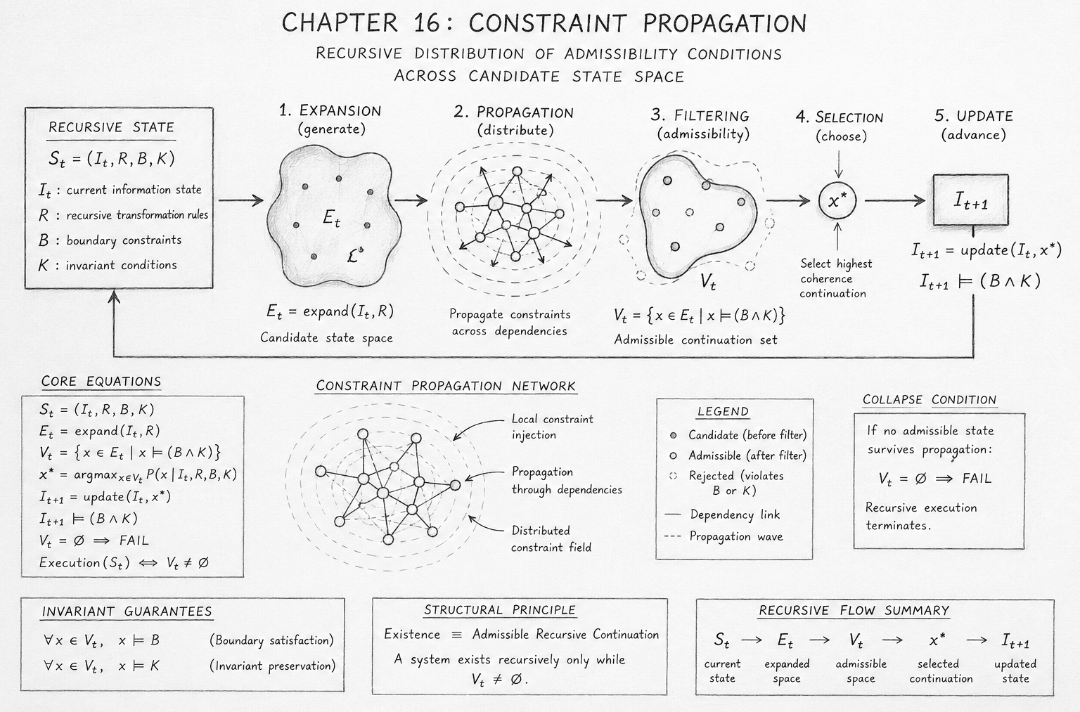
The Chapter 16 diagram illustrates constraint propagation as a recursive admissibility mechanism governing how coherent systems preserve structurally valid continuation across evolving state space. The diagram presents recursive execution not as unrestricted computation, but as dynamically constrained survivability filtering operating across candidate future states.

The entire structure visualizes the following recursive progression:

\[ S_t \rightarrow E_t \rightarrow V_t \rightarrow x^* \rightarrow I_{t+1} \]

This sequence represents the full recursive lifecycle of constraint propagation.

1. Recursive State Block

The leftmost block defines the recursive system state:

\[ S_t = (I_t, R, B, K) \]

This establishes the foundational structural configuration from which recursive evolution emerges.

The diagram identifies four governing components:

Component Structural Meaning
\( I_t \) Current informational state
\( R \) Recursive transformation rules
\( B \) Boundary constraints
\( K \) Invariant-preservation conditions

This block serves as the origin of recursive continuation generation.

The system cannot evolve independently from these structural conditions because every future state remains constrained by them throughout recursive propagation.

2. Expansion Region — Candidate State Space

The first major transformation stage is the expansion field:

\[ E_t = \operatorname{expand}(I_t, R) \]

The shaded irregular geometry represents recursive possibility space.

Each internal node symbolizes a potential future continuation generated from the current recursive configuration.

Importantly, the diagram intentionally depicts this space as:

  • dense,
  • unfiltered,
  • partially unordered,
  • structurally unconstrained prior to propagation.

This visualizes the fact that recursive expansion over-generates candidate trajectories before admissibility filtering occurs.

The expansion stage therefore represents possibility generation rather than validity.

3. Propagation Network

The central propagation structure illustrates recursive constraint distribution across dependency networks.

The interconnected graph demonstrates that:

  • constraints do not remain localized,
  • admissibility conditions propagate recursively,
  • local violations influence surrounding regions,
  • coherence conditions distribute through dependency links.

The outward wavefront rings represent propagated structural influence fields.

These rings symbolize recursive dissemination of:

  • boundary conditions,
  • invariant requirements,
  • admissibility restrictions,
  • contradiction pressure.

This portion of the diagram is critical because it visualizes propagation as a distributed recursive field rather than a linear validation step.

Constraint propagation reshapes the geometry of future continuation itself.

4. Filtering Region — Admissible Continuation Space

The next region visualizes admissibility filtering:

\[ V_t = \{x \in E_t \mid x \models (B \land K)\} \]

The filtered geometry is visibly reduced compared to the original expansion region.

This reduction illustrates recursive elimination of structurally invalid continuations.

The diagram differentiates between:

  • surviving admissible states,
  • rejected inconsistent states.

Rejected states appear outside the admissible region, symbolizing recursive exclusion caused by:

  • boundary violations,
  • invariant violations,
  • contradiction propagation,
  • coherence failure.

This section demonstrates that recursive systems do not evolve through unrestricted state traversal.

They evolve only through structurally survivable continuation regions.

5. Continuation Selection

The isolated node labeled:

\[ x^* \]

represents the selected recursive continuation.

The diagram associates this stage with:

\[ x^* = \operatorname*{arg\,max}_{x \in V_t} P(x \mid I_t, R, B, K) \]

This indicates that among all admissible continuations, the system selects the highest-coherence survivable trajectory.

The diagram intentionally isolates the selected continuation visually to emphasize:

  • coherence concentration,
  • admissibility stabilization,
  • recursive commitment to continuation.

Selection therefore represents the stabilization of recursive survival.

6. Recursive Update Block

The final update block represents recursive state advancement:

\[ I_{t+1} = \operatorname{update}(I_t, x^*) \]

This transforms the selected admissible continuation into the next recursive informational state.

The diagram also includes the coherence guarantee:

\[ I_{t+1} \models (B \land K) \]

This indicates that recursive continuation preserves all propagated structural requirements.

The update block therefore visualizes successful recursive survival.

7. Collapse Condition Panel

The collapse condition section formalizes recursive termination:

\[ V_t = \varnothing \;\Rightarrow\; \mathrm{FAIL} \]

This panel is structurally important because it establishes that:

  • recursive continuation is conditional,
  • existence depends on admissible continuation availability,
  • recursive systems terminate when propagation eliminates all survivable futures.

The diagram therefore defines collapse as structural non-survivability rather than procedural interruption.

8. Core Equation Panel

The equation panel summarizes the complete recursive propagation structure:

\[ S_t = (I_t, R, B, K) \]

\[ E_t = \operatorname{expand}(I_t, R) \]

\[ V_t = \{x \in E_t \mid x \models (B \land K)\} \]

\[ x^* = \operatorname*{arg\,max}_{x \in V_t} P(x \mid I_t, R, B, K) \]

\[ I_{t+1} = \operatorname{update}(I_t, x^*) \]

This panel mathematically compresses the full recursive execution pipeline into a compact formal system.

9. Invariant Guarantee Section

The lower-left invariant section illustrates preserved recursive structural identities:

  • \[ \forall x \in V_t,\; x \models B \]
  • \[ \forall x \in V_t,\; x \models K \]

These guarantees ensure that all surviving continuations preserve:

  • recursive boundaries,
  • coherence conditions,
  • structural identity consistency.

This section visualizes propagation as a coherence-preserving mechanism.

10. Structural Principle Panel

The center-bottom section presents the core ontological statement:

Existence≡Admissible Recursive Continuation

This is the foundational philosophical principle of the entire diagram.

The system exists recursively only while structurally admissible future states remain available.

Constraint propagation therefore governs:

  • recursive survival,
  • coherence preservation,
  • structural stability,
  • continuation existence itself.

11. Recursive Geometry Interpretation

Geometrically, the diagram represents recursive evolution as constrained traversal through admissibility topology.

The recursive system:

  • expands into possibility space,
  • propagates structural restrictions,
  • collapses invalid regions,
  • stabilizes coherent trajectories,
  • advances through survivable continuation geometry.

Constraint propagation therefore shapes the topology of recursive future evolution.

The diagram visualizes this as a dynamic filtering geometry rather than a procedural algorithm.

12. Overall Scientific Meaning

The complete diagram demonstrates that recursive systems survive not because they generate arbitrary futures, but because structurally invalid continuations are recursively eliminated through propagated coherence constraints.

Constraint propagation therefore acts as:

  • a recursive stability mechanism,
  • an admissibility enforcement field,
  • a contradiction elimination process,
  • a coherence-preserving geometry,
  • and a foundational law governing recursive existence itself.

Diagram → Flow Mapping Table

Diagram Component Flow Algebra Section Structural Meaning Mathematical Mapping
Recursive State Block state Defines the complete recursive system configuration \( S_t = (I_t, R, B, K) \)
Information State (\( I_t \)) state.I_t Current recursive informational structure \( I_t \)
Recursive Rules (\( R \)) state.R Transformation laws governing expansion \( R \)
Boundary Constraints (\( B \)) state.B Structural limits restricting admissibility \( B \)
Invariant Conditions (\( K \)) state.K Preserved recursive identities \( K \)
Expansion Field expand Generates candidate recursive continuations \( E_t = \operatorname{expand}(I_t, R) \)
Candidate Nodes expand.output Possible future recursive states \( x \in E_t \)
Expansion Geometry expand.meaning Recursive possibility space before filtering \( E_t \)
Propagation Network propagate_constraints Distributes admissibility conditions recursively \( x \models (B \land K) \)
Dependency Links propagate_constraints.across Structural coupling between candidate states \( \Delta B_i \Rightarrow \Delta V_{t+n} \)
Propagation Waves monitors.propagation_failure Recursive spread of structural influence \( \mathcal{C}(E_t) \)
Constraint Injection Arrows constraints Boundary and invariant enforcement \( (B \land K) \)
Filtering Region filter Removes structurally invalid states \( V_t = \{ x \in E_t \mid x \models (B \land K) \} \)
Surviving Nodes filter.output Admissible recursive continuations \( x \in V_t \)
Rejected Nodes monitors.boundary_violation States violating propagated constraints \( x \not\models (B \land K) \Rightarrow x \notin V_t \)
Reduced Geometry Shape filter.meaning Admissible continuation topology \( V_t \subseteq E_t \)
Selection Node (\( x^* \)) select.output Highest-coherence survivable continuation \( x^* = \arg\max_{x \in V_t} P(x \mid I_t, R, B, K) \)
Selection Arrows select Recursive continuation stabilization \( x^* \in V_t \)
Update Block (\( I_{t+1} \)) update.output Next coherent recursive informational state \( I_{t+1} = \operatorname{update}(I_t, x^*) \)
Update Guarantee update.guarantee Preservation of propagated admissibility \( I_{t+1} \models (B \land K) \)
Collapse Panel collapse Recursive termination condition \( V_t = \varnothing \Rightarrow \mathrm{FAIL} \)
Collapse Statement collapse.meaning No admissible continuation survives \( \text{Execution terminates} \)
Execution Condition execution Recursive existence depends on admissibility \( \mathrm{Execution}(S_t) \Leftrightarrow V_t \neq \varnothing \)
Invariant Guarantee Box invariants Preserves structural identities during continuation \( \forall x \in V_t,\; x \models K \)
Boundary Guarantee Box invariants.admissibility Preserves recursive structural limits \( \forall x \in V_t,\; x \models B \)
Structural Principle Panel summary.statement Recursive existence equals admissible continuation \( \mathrm{Existence} \equiv (V_t \neq \varnothing) \)
Recursive Flow Summary output.success Full recursive propagation lifecycle \( S_t \rightarrow E_t \rightarrow V_t \rightarrow x^* \rightarrow I_{t+1} \)
Entire Diagram Structure flow Unified recursive constraint propagation system \( O = R(I) \mid (B, K) \)
Full Geometric Interpretation summary Recursive evolution constrained by admissibility topology \( \mathcal{A}(S_t) \subseteq E_t \)
Constraint Stability Condition fixed_structure Stable rules produce stable admissibility space \( (I_t, R, B, K)\ \text{fixed} \Rightarrow V_t\ \text{fixed} \)
Global Coherence Region invariants.coherence Recursive continuation preserves distributed structure \( \forall x_i \in V_t,\; \bigcup_i x_i \models (B \land K) \)

Execution Guarantee Statement

Constraint Propagation

The Constraint Propagation flow guarantees that recursive execution proceeds only through structurally admissible continuations that satisfy all propagated boundary and invariant conditions.

Execution is formally defined by the existence of at least one valid recursive continuation:

\[ \mathrm{Execution}(S_t) \;\Longleftrightarrow\; V_t \neq \varnothing \]

where:

\[ V_t = \{x \in E_t \mid x \models (B \land K)\} \]

This guarantees that every surviving continuation:

  • satisfies all propagated boundary constraints,
  • preserves all invariant conditions,
  • remains recursively coherent,
  • and supports structurally valid continuation.

The flow enforces recursive admissibility preservation through distributed constraint propagation across all candidate future states.

For every surviving continuation:

\[ \forall x \in V_t,\; x \models B \]

\[ \forall x \in V_t,\; x \models K \]

Thus, no recursive state violating propagated structural requirements may advance execution.

The recursive update mechanism further guarantees coherence preservation during state transition:

\[ I_{t+1} = \operatorname{update}(I_t, x^*) \]

subject to:

\[ I_{t+1} \models (B \land K) \]

This ensures that successful recursive continuation preserves:

  • structural consistency,
  • admissibility stability,
  • recursive boundary integrity,
  • invariant continuity.

The flow additionally guarantees deterministic admissibility under fixed recursive conditions:

\[ (I_t, R, B, K)\ \text{fixed} \;\Rightarrow\; V_t\ \text{fixed} \]

Therefore:

  • identical recursive conditions yield identical admissible continuation spaces,
  • propagation behavior remains structurally reproducible,
  • recursive survivability remains mathematically stable.

The system also guarantees automatic contradiction elimination.

Any candidate continuation violating propagated structural constraints is recursively excluded:

\[ x \not\models (B \land K) \;\Rightarrow\; x \notin V_t \]

Thus, invalid recursive trajectories cannot propagate into future execution states.

If propagation eliminates all admissible continuations, recursive execution terminates immediately:

\[ V_t = \varnothing \;\Rightarrow\; \mathrm{FAIL} \]

This collapse condition guarantees that structurally inconsistent recursive states cannot continue execution artificially.

The flow therefore guarantees:

  • recursive admissibility enforcement,
  • propagated coherence preservation,
  • contradiction elimination,
  • invariant continuity,
  • recursive survivability validation,
  • deterministic structural filtering,
  • and stable recursive continuation.

The complete execution guarantee may therefore be summarized as:

\[ S_t \rightarrow E_t \rightarrow V_t \rightarrow x^* \rightarrow I_{t+1} \]

subject always to:

\[ V_t \neq \varnothing \]

and:

\[ \forall x \in V_t,\; x \models (B \land K) \]

The Constraint Propagation flow therefore guarantees that recursive systems evolve only through structurally survivable continuations consistent with all propagated coherence requirements.

Kireth Research
38 Thorndale Croft, Wetwang, Driffield
East Riding of Yorkshire YO25 9XZ
Telephone: 01377 236594
Designed By