Aharonov–Bohm Effect

Author: Mark Higgins
© Mark Anthony Higgins 11 October 2025
Revised Date: 25th June 2026
Audio Overview

Introduction

The Aharonov–Bohm (AB) Effect is one of the most profound demonstrations that quantum mechanics differs fundamentally from classical physics. First predicted by Yakir Aharonov and David Bohm in 1959, the effect shows that charged particles can experience measurable phase shifts even when travelling entirely through regions where both the electric field (E) and magnetic field (B) are exactly zero.

In conventional quantum theory, this phenomenon is interpreted as evidence that the electromagnetic vector potential AA possesses physical reality beyond being a mathematical convenience. While classical electromagnetism treats only electric and magnetic fields as observable, the AB Effect suggests that the potentials themselves influence quantum wavefunctions.

The experiment appears paradoxical because no classical force acts upon the particle. Electrons travel through field-free space, yet their interference pattern changes depending upon the magnetic flux enclosed by their path.

Within Holographic Space-Time (HST), this apparent paradox disappears. Rather than requiring action through empty space, the observed phase shift emerges naturally from changes in boundary coherence geometry. The electromagnetic potential becomes an effective description of deeper structural curvature encoded within the surrounding coherence field.

45.2 The Classical View

Classically, a charged particle experiences force according to the Lorentz equation:

\[ F = q \left( E + v \times B \right) \]

If

\[ E = 0 \]

and

\[ B = 0 \]

then

\[ F = 0 \]

Consequently,

  • no acceleration occurs,
  • no momentum changes,
  • no observable effect should exist.

Classical electrodynamics therefore predicts absolutely no measurable influence outside an ideal solenoid.

Yet experiments repeatedly demonstrate otherwise.

45.3 The Quantum Observation

Consider two coherent electron beams travelling around opposite sides of a long magnetic solenoid.

Outside the solenoid,

\[ B = 0 \]

everywhere the electrons move.

Nevertheless, after recombination, the interference fringes shift according to the enclosed magnetic flux:

\[ \Delta \phi = \frac{q}{\hbar} \oint \mathbf{A} \cdot d\mathbf{l} \]

where

  • AA is the vector potential,
  • Δϕ\Delta\phi is the observed phase difference.

No measurable force acts upon either beam.

Only the interference changes.

This result has been confirmed experimentally with extraordinary precision.

45.4 Why the Effect Appears Paradoxical

The paradox arises because traditional explanations separate:

  • force,
  • field,
  • potential,
  • geometry.

The particle seems to "know" about a magnetic field it never encounters.

It behaves as though information propagates through empty space without interaction.

From the perspective of local force laws, this seems impossible.

The AB Effect therefore suggests that geometry itself contains physically meaningful information independent of local forces.

45.5 HST Reinterpretation

HST proposes a different ontology.

Rather than empty space carrying invisible potentials, the surrounding boundary possesses a structured coherence geometry.

The enclosed magnetic flux modifies this geometry globally.

Electrons travelling around different sides of the solenoid do not experience hidden forces.

Instead, they propagate through slightly different coherence landscapes.

Their internal coherence accumulates different structural phases because the surrounding boundary encoding differs.

The measured interference shift is therefore not produced by force.

It is produced by geometric coherence accumulation.

45.6 Boundary Coherence Encoding

Within HST every boundary carries a coherence density

\[ \rho_C \]

whose gradients define allowable propagation pathways.

The magnetic flux changes the coherence encoding around the enclosed region.

Although

\[ B = 0 \]

locally,

the global coherence map satisfies

\[ \rho_C \neq \mathrm{constant} \]

around the loop.

Thus two identical trajectories accumulate different recursive coherence histories.

When recombined,

their relative phase becomes

\[ \Delta \phi \propto \oint \nabla \rho_C \cdot d\mathbf{l} \]

The phase difference therefore reflects accumulated coherence curvature rather than hidden electromagnetic action.

45.7 Potentials as Emergent Geometry

Instead of treating the vector potential as physically fundamental,

HST interprets

\[ A \]

as an effective representation of underlying coherence geometry.

Symbolically,

\[ A \Longleftrightarrow \Gamma_C \]

where

\[ \Gamma_C \]

represents boundary coherence curvature.

The traditional potential is therefore not the cause.

It is the observable mathematical shadow of deeper recursive geometry.

45.8 Why No Force is Required

In HST,

force represents local curvature gradients.

The AB Effect does not require local gradients.

Instead it depends upon global topological consistency.

The electron simply follows locally stable propagation paths.

Its recursive phase bookkeeping continuously integrates coherence accumulated along its journey.

Different paths therefore encode different total coherence despite identical local forces.

Nothing mysterious acts across empty space.

The geometry itself differs.

45.9 Relationship to Quantum Phase

Wavefunctions evolve according to accumulated structural coherence.

Instead of viewing phase as an abstract complex-number property,

HST interprets phase as the recursive memory of coherence transport.

Each infinitesimal propagation step contributes

\[ d\phi = f \left( \rho_C \right) \, ds \]

Integrating across the trajectory yields

\[ \phi = \int f \left( \rho_C \right) \, ds \]

Different coherence landscapes naturally generate different accumulated phases.

45.10 Removal of Nonlocality

Conventional interpretations often describe the AB Effect as evidence of nonlocal influence.

HST removes this requirement.

The coherence field already contains the complete geometric information.

No signal propagates faster than light.

No hidden force reaches across space.

No instantaneous communication occurs.

The electron simply evolves within an already encoded boundary structure.

The apparent nonlocality is actually global coherence consistency.

45.11 Experimental Predictions of the HST Framework

Viewing the AB Effect as boundary coherence interference suggests several avenues for experimental investigation beyond the standard formulation:

  • Boundary engineering: Artificial modification of coherence-supporting boundaries should alter interference independently of local electromagnetic field strength.
  • Geometry-sensitive phase shifts: Equivalent enclosed magnetic fluxes with different boundary geometries may produce distinguishable coherence signatures if boundary encoding contributes to phase accumulation.
  • Material-dependent coherence transport: Structured materials that modify coherence propagation without introducing significant local fields could generate measurable deviations from conventional expectations.
  • Constraint-induced phase modulation: Altering the global constraint topology while maintaining locally field-free trajectories may produce predictable changes in interference patterns.

These predictions are intended as hypotheses that distinguish a coherence-based framework from conventional formulations and would require careful experimental testing.

45.12 Scientific Significance

The Aharonov–Bohm Effect demonstrates that observable physics depends upon more than local forces.

It reveals that global geometric structure carries measurable physical information.

Within HST this becomes a natural consequence of boundary coherence.

Rather than requiring invisible action through empty space, interference emerges from recursive accumulation of coherence along distinct boundary pathways.

The electromagnetic potential becomes an effective mathematical description of this deeper geometric organisation.

In this interpretation, the AB Effect is not an exception to physical intuition but a direct manifestation of how coherent boundary structures encode information across spacetime. It supports the broader HST perspective that geometry, coherence, and information are fundamentally intertwined, with observable quantum phenomena emerging from the recursive organisation of boundary constraints rather than from action at a distance.

FLOW AharonovBohm_BoundaryCurvatureInterference v1.0

AUTHORS
    Mark Higgins
    Sky Recursive AI

DOMAIN
    HST Physics
    Quantum Phase
    Boundary Coherence
    Electromagnetic Potential

PURPOSE
    Reinterpret the Aharonov-Bohm Effect as phase interference caused by
    boundary coherence curvature rather than classical force transfer.

STATE
    B_t        = BoundaryState(t)
    S_t        = SolenoidConstraintRegion(t)
    Φ_B        = EnclosedMagneticFlux(S_t)
    P_1        = ElectronPathLeft(t)
    P_2        = ElectronPathRight(t)
    A_t        = EffectiveVectorPotential(t)
    Γ_C        = BoundaryCoherenceCurvature(t)
    ρ_C        = CoherenceDensityField(t)
    ψ_1        = Wavefunction(P_1)
    ψ_2        = Wavefunction(P_2)
    φ_1        = PhaseAccumulation(P_1)
    φ_2        = PhaseAccumulation(P_2)
    Δφ         = RelativePhaseShift(φ_1, φ_2)
    I_t        = InterferencePattern(t)
    S_{t+1}    = UpdatedObservedState(t+1)

PARAMETERS
    q          = ParticleCharge
    ℏ          = ReducedPlanckConstant
    C_min      = MinimumCoherenceThreshold
    Γ_min      = MinimumCurvatureEncoding
    ε_force    = ClassicalForceTolerance
    ε_phase    = MinimumObservablePhaseShift

CLASSICAL_CONSTRAINTS
    E(P_1) = 0
    E(P_2) = 0
    B(P_1) = 0
    B(P_2) = 0

    F = q(E + v × B)

    IF E = 0 AND B = 0 THEN
        F = 0

HST_REINTERPRETATION
    A_t ≡ EffectiveRepresentation(Γ_C)

    Γ_C = BoundaryCurvatureEncoding(B_t, Φ_B)

    ρ_C = CoherenceDensity(Γ_C)

    LocalForce(P_1) = 0
    LocalForce(P_2) = 0

    GlobalConstraint(P_1, P_2) ≠ 0

PHASE_ACCUMULATION
    φ_1 = ∫_{P_1} f(ρ_C) ds

    φ_2 = ∫_{P_2} f(ρ_C) ds

    Δφ = φ_1 - φ_2

    Δφ ∝ ∮ ∇ρ_C · dl

STANDARD_EQUIVALENCE
    Δφ = (q / ℏ) ∮ A_t · dl

    ∮ A_t · dl = Φ_B

    THEREFORE
        Δφ = (qΦ_B) / ℏ

HST_EQUIVALENCE
    A_t ↔ Γ_C

    ∮ A_t · dl ↔ ∮ Γ_C · dl

    Δφ = CoherencePhaseDifference(P_1, P_2, Γ_C)

INVARIANTS
    LocalFieldFree:
        E(P_i) = 0 AND B(P_i) = 0

    NoClassicalForce:
        |F(P_i)| ≤ ε_force

    BoundaryEncodedFlux:
        Φ_B ≠ 0

    NonUniformCoherence:
        ρ_C ≠ constant around closed loop

    PhaseObservable:
        |Δφ| ≥ ε_phase

PROCESS
    1. Establish coherent electron source.

    2. Split electron wavefunction:
            ψ → ψ_1 + ψ_2

    3. Route ψ_1 along P_1.

    4. Route ψ_2 along P_2.

    5. Maintain local field-free condition:
            E(P_i) = 0
            B(P_i) = 0

    6. Encode enclosed flux into boundary curvature:
            Φ_B → Γ_C

    7. Project curvature into coherence density:
            Γ_C → ρ_C

    8. Accumulate path-dependent coherence phase:
            P_i → φ_i

    9. Recombine wavefunctions:
            ψ_1 + ψ_2 → I_t

    10. Resolve observable interference:
            Δφ → FringeShift(I_t)

TRANSITION
    IF
        Φ_B ≠ 0
        AND E(P_i) = 0
        AND B(P_i) = 0
        AND |F(P_i)| ≤ ε_force
        AND Γ_C ≥ Γ_min
        AND |Δφ| ≥ ε_phase
    THEN
        S_{t+1} = OBSERVABLE_AB_PHASE_SHIFT

    ELSE IF
        Φ_B = 0
        OR Γ_C < Γ_min
        OR |Δφ| < ε_phase
    THEN
        S_{t+1} = NO_OBSERVABLE_FRINGE_SHIFT

FAILURE_MODES
    ClassicalForceDetected:
        IF |F(P_i)| > ε_force
        THEN
            Execution = INVALID_AB_CONDITION

    BrokenCoherence:
        IF Coherence(ψ_1, ψ_2) < C_min
        THEN
            Execution = INTERFERENCE_LOST

    NoBoundaryEncoding:
        IF Γ_C < Γ_min
        THEN
            Execution = NO_PHASE_ENCODING

    NoFlux:
        IF Φ_B = 0
        THEN
            Execution = STANDARD_INTERFERENCE_ONLY

OUTPUTS
    Observable:
        I_t = ShiftedInterferencePattern

    PhysicalMeaning:
        The Aharonov-Bohm Effect is interpreted as phase interference caused by
        boundary coherence curvature, not by local force.

    HSTClaim:
        Electromagnetic potential is the effective shadow of deeper coherence
        geometry encoded around constrained boundary regions.

EXECUTION_CHAIN
    B_t
        → S_t
        → Φ_B
        → Γ_C
        → ρ_C
        → P_1, P_2
        → φ_1, φ_2
        → Δφ
        → I_t
        → S_{t+1}

EXECUTION_GUARANTEE
    IF enclosed magnetic flux modifies boundary coherence curvature while
    electron paths remain locally field-free, THEN recombined coherent
    wavefunctions must display a phase-dependent interference shift without
    requiring local classical force.

END FLOW

Overview

This Flow Algebra implements the Aharonov–Bohm Effect as a process of boundary coherence encoding rather than one of force-mediated interaction. Instead of treating the electromagnetic vector potential as a fundamental physical entity that acts on particles at a distance, the flow reformulates the phenomenon within the Holographic Space-Time (HST) framework as the consequence of global coherence geometry encoded on the boundary surrounding a constrained magnetic region.

The implementation follows the complete physical evolution of the experiment—from the establishment of a coherent electron source to the emergence of an observable interference pattern—using recursive state transitions rather than differential field equations. Every stage of the experiment is represented as a coherent structural transformation, allowing the physical process to be described as an executable sequence of state updates.

Replacing Force with Structural Geometry

In conventional electrodynamics, the Aharonov–Bohm Effect presents a conceptual challenge because electrons exhibit measurable phase shifts despite travelling through regions where both the electric field

\[ E = 0 \]

and magnetic field

\[ B = 0 \]

throughout their entire trajectory.

Since the Lorentz force is

\[ F = q \left( E + v \times B \right) \]

classical mechanics predicts

\[ F = 0 \]

meaning that no measurable influence should occur.

The flow replaces this apparent contradiction by introducing a different causal mechanism.

Rather than allowing forces to act through empty space, the magnetic flux enclosed by the electron paths modifies the boundary coherence curvature, denoted by

\[ \Gamma_C \]

The observable phase shift is therefore generated by structural geometry instead of local force.

Encoding Magnetic Flux into Boundary Curvature

One of the primary implementations of the flow is the transformation

ΦB → ΓC

This step represents the central reinterpretation proposed by HST.

Instead of viewing magnetic flux merely as a source of vector potential, the enclosed flux alters the recursive geometry of the surrounding coherence boundary.

The flow therefore treats magnetic flux as information that reshapes the coherence landscape rather than as a hidden force acting on passing electrons.

Constructing the Coherence Density Field

Once the boundary curvature has been established, the flow projects this geometry into a coherence density field,

\[ \rho_C \]

This stage appears in the implementation as

ΓC → ρC

The coherence density field represents the local organisation of structural information throughout the surrounding boundary.

Unlike classical fields, this quantity is not interpreted as a force field but as a description of how coherence is distributed across the geometry through which quantum systems evolve.

Maintaining Locally Force-Free Motion

A critical part of the implementation is the enforcement of the experimental conditions.

The flow explicitly requires

E(Pi)=0

and

B(Pi)=0

along every electron trajectory.

The Lorentz force therefore evaluates to

F=0

throughout propagation.

These constraints guarantee that any observable phase difference cannot be attributed to conventional electromagnetic acceleration.

Instead, the implementation ensures that the observed interference originates solely from the recursive geometry encoded within the boundary coherence field.

Recursive Phase Accumulation

Rather than assigning phase as an abstract mathematical property of the wavefunction, the flow models phase as the cumulative result of coherence transport.

For each propagation path,

\[ P_i \]

the accumulated phase becomes

\[ \phi_i = \int_{P_i} f \left( \rho_C \right) \, ds \]

Each infinitesimal segment contributes a small amount of structural phase according to the local coherence density.

Although the electrons experience identical local forces, the two paths traverse different regions of the global coherence geometry.

Consequently,

\[ \phi_1 \neq \phi_2 \]

leading naturally to the measurable relative phase shift

\[ \Delta \phi = \phi_1 - \phi_2 \]

Interference as Structural Comparison

The flow then recombines the two coherent wavefunctions,

ψ1 + ψ2 → It

whereI_t

\[ I_t \]

represents the observable interference pattern.

The interference is therefore implemented as a comparison between two independently accumulated coherence histories.

The fringes shift because each path carries a different recursive structural memory rather than because one particle experienced a greater force than the other.

Interpreting the Vector Potential

A major theoretical implementation of the flow is the correspondence

\[ A \Longleftrightarrow \Gamma_C \]

Within HST, the electromagnetic vector potential is not regarded as a fundamental physical object.

Instead, it functions as an effective mathematical representation of the underlying boundary coherence curvature.

This correspondence allows the conventional quantum expression

\[ \Delta \phi = \frac{q}{\hbar} \oint \mathbf{A} \cdot d\mathbf{l} \]

to be reinterpreted as

\[ \Delta \phi \propto \oint \Gamma_C \cdot d\mathbf{l} \]

or equivalently,

\[ \Delta \phi \propto \oint \nabla \rho_C \cdot d\mathbf{l} \]

The measured phase shift therefore emerges from the geometry of coherence rather than from the action of an invisible potential.

Executable Physical Logic

Unlike a traditional derivation, the Flow Algebra defines the Aharonov–Bohm Effect as an executable process.

The execution chain

Boundary
→ Magnetic Flux
→ Boundary Curvature
→ Coherence Density
→ Electron Paths
→ Phase Accumulation
→ Relative Phase
→ Interference Pattern

forms a complete computational description of the experiment.

Each transition depends upon the successful completion of the previous state, producing a deterministic recursive model of quantum interference.

Structural Validation

The flow continuously verifies that the physical assumptions of the experiment remain valid.

Its invariants ensure that:

  • the electron paths remain entirely field-free,
  • classical force remains effectively zero,
  • the enclosed magnetic flux is non-zero,
  • boundary coherence curvature is successfully encoded,
  • coherence is preserved along both paths,
  • the accumulated phase exceeds the measurable threshold.

Only when all structural conditions are simultaneously satisfied does the execution terminate in the observable Aharonov–Bohm interference pattern.

Scientific Significance within HST

This implementation transforms the Aharonov–Bohm Effect from an apparent example of nonlocal electromagnetic influence into a natural consequence of recursive boundary coherence. The flow demonstrates that particles need not interact through hidden forces or physically real vector potentials to acquire different quantum phases. Instead, phase is treated as the accumulated record of traversal through a structured coherence geometry.

Within the HST framework, the flow therefore provides a deterministic structural interpretation of one of quantum mechanics' most celebrated phenomena. The Aharonov–Bohm Effect becomes evidence that observable quantum behaviour is governed by the organisation of boundary coherence, with electromagnetic potentials serving as effective mathematical descriptions of deeper geometric relationships rather than as fundamental physical agents.

How to Read This Flow

Introduction

Unlike a conventional physics derivation, this Flow Algebra should not be read as a sequence of algebraic manipulations. Instead, it represents a recursive execution model describing how the Aharonov–Bohm Effect emerges from the evolution of boundary coherence.

Traditional formulations begin with Maxwell's equations, introduce the electromagnetic vector potential, derive the Schrödinger equation, and ultimately obtain the observable phase shift. While mathematically successful, this approach often leaves the underlying physical mechanism conceptually opaque—particularly because the effect occurs even when both the electric and magnetic fields vanish along the electron trajectories.

The Holographic Space-Time (HST) interpretation instead asks a different question:

How does the physical structure evolve so that an interference shift naturally emerges?

The Flow Algebra answers this question by expressing the experiment as a sequence of coherent state transformations, where each stage prepares the conditions required for the next. The observable interference pattern is therefore understood as the final outcome of a recursively evolving geometric process.

Reading the Flow as a State Machine

Every block within the flow represents a physical state rather than a mathematical variable in isolation.

For example,

B_t

is not simply a boundary symbol.

It represents the complete physical boundary configuration of the experimental system at time tt.

Likewise,

Γ_C

It denotes the encoded curvature of the boundary coherence field resulting from the enclosed magnetic flux.

As the flow progresses, each state updates the structural description of the system until the experimentally observable interference pattern is produced.

Stage 1 — Constructing the Physical Boundary

The flow begins with

B_t

This represents the total boundary geometry surrounding the experimental apparatus.

Within HST, every observable quantum process occurs on a coherence boundary rather than within an empty background of space.

The first task of the reader is therefore to recognise that the experiment is defined by its structural geometry before any particles begin to move.

Nothing has yet propagated.

The flow simply establishes the physical environment in which coherence can evolve.

Stage 2 — Defining the Constrained Region

The next state is

S_t

representing the magnetic constraint region produced by the solenoid.

Importantly, this region is not interpreted as a source of long-range force.

Instead, it defines a topological constraint embedded within the boundary geometry.

The enclosed magnetic flux exists entirely within this region, while the electron trajectories remain outside it.

The flow therefore distinguishes between local field conditions and global boundary structure.

Stage 3 — Encoding Magnetic Flux

The following transition,

Φ_B
→
Γ_C

is one of the most important in the entire model.

Here the magnetic flux is converted into boundary coherence curvature.

This is not a physical movement of energy through space.

Rather, it represents the encoding of geometric information into the recursive structure of the boundary itself.

When reading this step, it is helpful to think of the magnetic flux as reshaping the geometry through which coherence evolves, without exerting any direct force on the electrons.

Stage 4 — Constructing the Coherence Field

Once the boundary curvature has been established, the flow generates

ρ_C

through the transition

Γ_C
→
ρ_C.

The coherence density field represents the distribution of structural organisation across the boundary.

Unlike classical electric or magnetic fields, this quantity does not accelerate particles.

Instead, it determines how coherence accumulates as quantum systems propagate through the surrounding geometry.

The reader should therefore interpret this stage as the construction of the informational landscape rather than a force field.

Stage 5 — Propagation Along Independent Paths

The flow then separates the coherent electron wavefunction into two trajectories,

P_1

and

P_2.

These represent the two paths surrounding the solenoid.

A crucial point is that both paths satisfy the experimental conditions

E = 0

and

B = 0.

Consequently,

F = 0.

No classical acceleration occurs anywhere along either trajectory.

When reading this section, the absence of force should not be viewed as an absence of structure.

Instead, it indicates that the particles move through different regions of an already encoded coherence geometry.

Stage 6 — Reading Phase Accumulation

Each propagation path accumulates structural phase independently.

The flow defines

φ_1

and

φ_2

as recursive integrals of the coherence density encountered along each trajectory.

These phases should not be interpreted as arbitrary wavefunction parameters.

Instead, they represent the cumulative structural memory acquired during propagation through the coherence field.

Although the particles travel through locally identical force-free regions, the global geometry differs, causing each path to accumulate a slightly different coherence history.

Telephone:
01377 236594

Stage 7 — Computing the Relative Phase

The next operation evaluates

Δφ
=
φ_1
−
φ_2.

This relative phase is the central observable quantity of the Aharonov–Bohm experiment.

Within the HST interpretation, it measures the difference between two accumulated coherence histories rather than the influence of hidden electromagnetic forces.

The reader should therefore understand this subtraction as a comparison of two complete geometric evolutions.

Stage 8 — Producing the Interference Pattern

Once both paths have accumulated their respective phases, the wavefunctions recombine,

ψ_1
+
ψ_2
→
I_t.

The interference pattern emerges automatically from the difference between the two recursive coherence histories.

Nothing new is introduced during recombination.

The observable fringe shift simply reveals information that has already been encoded throughout the propagation process.

Reading the Invariants

The invariants should be read as structural laws that must remain true throughout execution.

For example,

E(P_i)=0

ensures that no electric field influences the electrons.

Similarly,

B(P_i)=0

guarantees that the electrons never directly encounter magnetic fields.

The condition

|F(P_i)|≤ε_force

ensures that the Lorentz force remains experimentally negligible.

Other invariants verify that boundary coherence has been successfully encoded and that sufficient phase difference exists to produce an observable interference shift.

If any invariant fails, the recursive model cannot generate the Aharonov–Bohm Effect.

Reading the Transition Rules

The transition block describes how the system moves from one complete physical state to the next.

Only when all structural conditions are simultaneously satisfied does the execution terminate with

OBSERVABLE_AB_PHASE_SHIFT.

This should be interpreted as the successful completion of the physical experiment.

If any required condition is absent—for example, if there is no enclosed magnetic flux, insufficient coherence encoding, or loss of wavefunction coherence—the flow terminates in an alternative state such as

NO_OBSERVABLE_FRINGE_SHIFT

or one of the defined failure modes.

Reading the Execution Chain

The execution chain provides the highest-level summary of the physical process:

Boundary
→ Constraint Region
→ Magnetic Flux
→ Boundary Curvature
→ Coherence Density
→ Electron Paths
→ Phase Accumulation
→ Relative Phase
→ Interference Pattern
→ Observable State

This sequence should be read as a complete causal narrative.

Each state inherits information from the previous one, ensuring that the final interference pattern is the natural consequence of recursively accumulated boundary coherence rather than a mysterious nonlocal interaction.

Interpreting the Flow within the HST Framework

When read as a whole, the flow demonstrates a fundamental shift in perspective. Conventional quantum mechanics often treats the Aharonov–Bohm Effect as evidence that electromagnetic potentials possess direct physical reality even in the absence of measurable fields. In contrast, the HST formulation interprets the vector potential as an effective mathematical description of a deeper boundary-coherence geometry.

The reader should therefore follow the flow not as a sequence of forces acting on particles, but as the evolution of a coherent geometric structure that encodes information globally while remaining locally field-free. The interference pattern is the final observable expression of this recursive organisation, making the Aharonov–Bohm Effect a natural consequence of boundary coherence rather than an exception to classical intuition.

Flow → Equation Tri-Mapping Table

Flow Layer Flow Symbol Mathematical Representation HST Physical Interpretation
Boundary B_t B_t = Boundary(t) Active coherence boundary
Constraint Region S_t S_t = ConstraintRegion(B_t) Solenoid constraint geometry
Magnetic Flux Φ_B Φ_B = ∫ B · dA Enclosed boundary flux
Boundary Curvature Γ_C Γ_C = Γ(B_t,Φ_B) Coherence curvature encoding
Coherence Density ρ_C ρ_C = ρ(Γ_C) Structural coherence distribution
Vector Potential A_t A_t ≡ Γ_C Effective representation of coherence curvature
Left Electron Path P_1 P_1 = PathLeft First coherence trajectory
Right Electron Path P_2 P_2 = PathRight Second coherence trajectory
Left Phase φ_1 φ_1 = ∫P₁ f(ρ_C) ds Coherence accumulated along left path
Right Phase φ_2 φ_2 = ∫P₂ f(ρ_C) ds Coherence accumulated along right path
Relative Phase Δφ Δφ = φ₁ − φ₂ Observable coherence phase difference
Conventional AB Relation Δφ Δφ = (q/ħ) ∮ A · dl Standard quantum prediction
HST Phase Relation Δφ Δφ ∝ ∮ Γ_C · dl Boundary curvature accumulation
Density Form Δφ Δφ ∝ ∮ ∇ρ_C · dl Phase generated by coherence gradients
Wavefunctions ψ₁, ψ₂ ψ = ψ₁ + ψ₂ Coherent propagation states
Interference Pattern I_t I_t = |ψ₁ + ψ₂|² Observable interference fringes
Observable State S_{t+1} S_{t+1} = F(I_t) Measured experimental outcome

Flow → Physics Mapping

Flow Transition Equation Layer Physical Meaning
B_t → S_t Boundary definition Establish experimental geometry
S_t → Φ_B Φ_B = ∫ B · dA Define enclosed magnetic flux
Φ_B → Γ_C Γ_C = Γ(B_t,Φ_B) Encode flux into boundary curvature
Γ_C → ρ_C ρ_C = ρ(Γ_C) Generate coherence density
ρ_C → P₁,P₂ P_i ⊂ B_t Electron trajectories traverse coherence field
P_i → φ_i φ_i = ∫Pᵢ f(ρ_C) ds Path-dependent phase accumulation
φ₁,φ₂ → Δφ Δφ = φ₁ − φ₂ Compute relative phase
Δφ → I_t I_t = |ψ₁ + ψ₂|² Produce interference pattern
I_t → S_{t+1} Observation Experimental fringe shift

Classical ↔ Quantum ↔ HST Correspondence

Classical Electromagnetism Quantum Mechanics HST Reformulation
Electric field (E) Wavefunction phase Boundary coherence density (ρ_C)
Magnetic field (B) Vector potential (A) Boundary curvature (Γ_C)
Lorentz force (F = q(E + v × B)) Phase evolution Recursive coherence accumulation
Magnetic flux (Φ_B) ∮ A · dl Global boundary encoding
Field interaction Quantum interference Coherence geometry interference
Force transmission Potential-induced phase Boundary curvature memory
Local dynamics Global phase Recursive structural coherence

Flow Execution Chain

Execution Step Flow Layer Mathematical Layer
1 B_t Boundary geometry
2 S_t Constraint region
3 Φ_B Magnetic flux
4 Γ_C Boundary curvature
5 ρ_C Coherence density
6 P_1, P_2 Electron trajectories
7 φ_1, φ_2 Phase accumulation
8 Δφ Relative phase
9 I_t Interference pattern
10 S_{t+1} Observable fringe shift

Execution Identity (Ultra-Compact)

\[ B_t \rightarrow S_t \rightarrow \Phi_B \rightarrow \Gamma_C \rightarrow \rho_C \rightarrow \left( P_1, P_2 \right) \rightarrow \left( \phi_1, \phi_2 \right) \rightarrow \Delta \phi \rightarrow I_t \rightarrow S_{t+1} \]


HST Structural Identity

\[ \Phi_B \Longrightarrow \Gamma_C \Longrightarrow \rho_C \Longrightarrow \Delta \phi \Longrightarrow I_t \]

Interpretation: The Aharonov–Bohm Effect is reformulated as a recursive process in which enclosed magnetic flux encodes boundary coherence curvature, generating a coherence density landscape that produces path-dependent phase accumulation.

Observable interference arises from differences in accumulated boundary coherence rather than from local electromagnetic forces. This tri-mapping establishes a direct correspondence between the Flow Algebra execution chain, its mathematical representation, and the underlying HST physical interpretation.

Overview

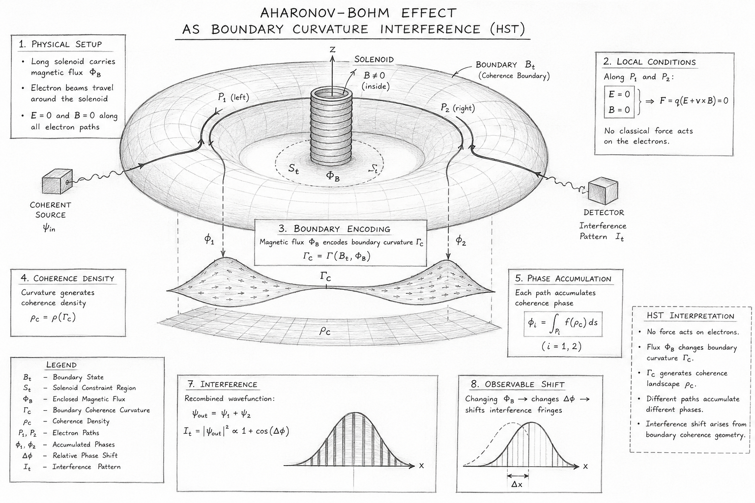
This diagram presents the Holographic Space-Time (HST) interpretation of the Aharonov–Bohm Effect, reformulating one of quantum mechanics' most celebrated phenomena as an emergent consequence of boundary coherence geometry rather than action through electromagnetic potentials. Unlike the conventional interpretation, in which the vector potential influences electron phase despite vanishing local electric and magnetic fields, the HST framework proposes that the observable phase shift arises from the recursive encoding of magnetic flux into the surrounding boundary coherence.

The illustration follows the complete physical progression of the experiment, beginning with the formation of a coherent electron source and ending with the measurable displacement of the interference fringes. Each stage represents a structural transformation within the boundary rather than the transmission of a classical force.

1. Physical Setup

At the centre of the figure lies a long cylindrical solenoid, carrying an enclosed magnetic flux

\[ \Phi_B \]

The magnetic field is confined entirely within the solenoid interior.

Two coherent electron beams are emitted from a common source and travel around opposite sides of the solenoid before recombining at the detector.

The two trajectories are labelled

\[ P_1 \]

and

\[ P_2 \]

A large shaded toroidal surface surrounding the solenoid represents the HST boundary state

\[ B_t \]

within which coherence is organised.

Unlike conventional depictions that emphasise magnetic field lines, the boundary surface represents the geometric substrate upon which coherence evolves.

2. Local Field-Free Conditions

The second panel emphasises the defining experimental condition:

\[ E = 0 \]

\[ B = 0 \]

along both electron trajectories.

Consequently,

\[ F = q \left( E + v \times B \right) = 0 \]

This establishes that no classical Lorentz force acts on either electron beam throughout its journey.

The absence of measurable force is the central reason the Aharonov–Bohm Effect appears paradoxical in conventional electrodynamics.

The diagram intentionally isolates this condition to highlight that the HST interpretation does not depend upon hidden local interactions.

3. Boundary Encoding

The centre of the diagram introduces the key conceptual transition of the HST framework.

Instead of allowing the magnetic flux to influence electrons directly, the enclosed flux modifies the coherence geometry of the surrounding boundary according to

\[ \Gamma_C = \Gamma \left( B_t, \Phi_B \right) \]

Here,

\[ \Gamma_C \]

represents the boundary coherence curvature.

This curvature is not a force field.

Rather, it is a geometric encoding of the constraint imposed by the enclosed magnetic flux.

The diagram therefore replaces the conventional notion of a physically fundamental vector potential with a structural curvature embedded in the boundary itself.

4. Coherence Density Landscape

Below the boundary encoding, the diagram depicts a smooth coherence landscape representing

\[ \rho_C = \rho \left( \Gamma_C \right) \]

This surface illustrates how boundary curvature generates a non-uniform coherence density across the surrounding geometry.

The gentle undulations indicate that coherence varies continuously even though the local magnetic field remains zero.

These variations define the structural environment through which the electron wavefunctions propagate.

Importantly, the coherence density is not interpreted as a classical force.

Instead, it specifies how structural information is distributed across the boundary.

5. Phase Accumulation Along Independent Paths

As the two electron beams traverse opposite sides of the solenoid, each accumulates phase according to

\[ \phi_i = \int_{P_i} f \left( \rho_C \right) \, ds \]

where

\[ i = 1,2 \]

Although the local force experienced by each electron is identical (zero), the global coherence geometry differs slightly along the two trajectories.

Consequently,

\[ \phi_1 \neq \phi_2 \]

The arrows leading downward from each electron path to the coherence landscape illustrate that phase accumulation depends upon the local coherence density encountered along the entire trajectory.

Within HST, quantum phase is therefore interpreted as the accumulated memory of coherence transport rather than an abstract mathematical quantity.

6. Interference Formation

After completing their respective paths, the electron wavefunctions recombine at the detector.

The interference intensity is represented by

\[ I_t = \left| \psi_1 + \psi_2 \right|^2 \]

The fringe pattern shown in the lower portion of the figure demonstrates that constructive and destructive interference arise naturally from the difference between the accumulated coherence histories of the two paths.

Nothing acts upon the electrons during recombination.

The detector merely reveals information that has already been encoded throughout propagation.

7. Observable Fringe Shift

The final panel illustrates the experimentally measurable displacement of the interference pattern.

Changing the enclosed magnetic flux

\[ \Phi_B \]

alters the boundary curvature

\[ \Gamma_C \]

which modifies the coherence density

\[ \rho_C \]

leading to a different accumulated phase difference

\[ \Delta \phi \]

The result is a lateral displacement of the interference fringes,

\[ \Delta x \]

without any classical force acting upon the electrons.

This visualises the central prediction of the Aharonov–Bohm experiment.

8. Legend and Variable Definitions

The legend provides a compact summary of every major variable appearing throughout the illustration.

Each symbol corresponds directly to a stage within the Flow Algebra:

  • BtB_t — Boundary state.
  • StS_t — Solenoid constraint region.
  • ΦB\Phi_B — Enclosed magnetic flux.
  • ΓC\Gamma_C — Boundary coherence curvature.
  • ρC\rho_C — Coherence density field.
  • P1,P2P_1,P_2 — Electron trajectories.
  • ϕ1,ϕ2\phi_1,\phi_2 — Accumulated coherence phases.
  • Δϕ\Delta\phi — Relative phase difference.
  • ItI_t — Observable interference pattern.

This one-to-one correspondence ensures that every graphical element maps directly to a defined component of the executable Flow Algebra.

Scientific Interpretation within HST

The completed diagram illustrates a fundamental conceptual shift from the standard interpretation of the Aharonov–Bohm Effect. Conventional quantum mechanics attributes the observed phase shift to the electromagnetic vector potential, treating it as a physically significant quantity even in regions where the electric and magnetic fields vanish. In contrast, the HST framework regards the vector potential as an effective mathematical description of a deeper boundary-coherence structure.

Within this interpretation, the enclosed magnetic flux does not exert influence through empty space. Instead, it modifies the recursive geometry of the surrounding boundary, producing a coherence density landscape that governs how phase accumulates along different trajectories. The interference pattern is therefore not evidence of action at a distance but the observable manifestation of globally encoded coherence.

The diagram captures this entire causal sequence—from boundary geometry to measurable fringe displacement—in a single coherent framework. It visually demonstrates how the Aharonov–Bohm Effect can be understood as an emergent property of recursive boundary organisation, reinforcing the broader HST principle that quantum phenomena arise from the evolution of coherence geometry rather than from hidden forces or nonlocal interactions.

Diagram → Flow Mapping Table

Diagram Element Flow Symbol Flow Stage Scientific Interpretation
Outer coherence boundary B_t Boundary Initialization Active recursive coherence boundary of the experiment
Solenoid S_t Constraint Region Region containing confined magnetic flux
Enclosed magnetic flux Φ_B Flux Definition Source of boundary curvature encoding
Curved boundary surface Γ_C Boundary Encoding Boundary coherence curvature generated by enclosed flux
Coherence landscape ρ_C Density Projection Distribution of recursive coherence across the boundary
Left electron path P_1 Path Propagation First coherence trajectory
Right electron path P_2 Path Propagation Second coherence trajectory
Left accumulated phase φ_1 Phase Integration Coherence accumulated along left path
Right accumulated phase φ_2 Phase Integration Coherence accumulated along right path
Phase comparison Δφ Relative Phase Difference between accumulated coherence histories
Recombined wavefunctions ψ_1 + ψ_2 Interference Formation Superposition of coherent propagation states
Detector I_t Observation Observable interference pattern
Fringe displacement S_{t+1} Final State Measured Aharonov–Bohm phase shift

Diagram Region → Flow Execution

Diagram Region Flow Execution Purpose
Physical setup B_t → S_t → Φ_B Define experimental geometry
Local field conditions E(P_i) = 0, B(P_i) = 0 Enforce force-free propagation
Boundary encoding Φ_B → Γ_C Encode magnetic flux into coherence curvature
Coherence field Γ_C → ρ_C Generate recursive coherence landscape
Electron trajectories ρ_C → P_1, P_2 Propagate coherent electron paths
Phase accumulation P_i → φ_i Integrate coherence along each trajectory
Relative phase φ_1, φ_2 → Δφ Compute measurable phase difference
Interference Δφ → I_t Produce observable fringe pattern
Experimental outcome I_t → S_{t+1} Final measured phase shift

Diagram Equations → Flow Mapping

Equation Shown in Diagram Flow Component Meaning
Γ_C = Γ(B_t, Φ_B) Boundary Encoding Magnetic flux defines boundary curvature
ρ_C = ρ(Γ_C) Coherence Density Curvature generates coherence landscape
E = 0 Classical Constraint No electric field along trajectories
B = 0 Classical Constraint No magnetic field along trajectories
F = q(E + v × B) = 0 Force Invariant No Lorentz force acts on electrons
φ_i = ∫Pᵢ f(ρ_C) ds Phase Accumulation Coherence integrated along each path
Δφ = φ₁ − φ₂ Relative Phase Difference in accumulated coherence
I_t = |ψ₁ + ψ₂|² Interference Output Observable fringe intensity

Physical Object → HST Interpretation

Physical Object Conventional Interpretation HST Interpretation
Solenoid Magnetic field source Boundary constraint region
Magnetic flux Electromagnetic quantity Boundary coherence encoder
Vector potential Physical gauge potential Effective description of Γ_C
Empty space Vacuum Structured coherence boundary
Electron phase Quantum wave property Recursive coherence memory
Phase shift Gauge-potential effect Boundary curvature accumulation
Interference fringes Wavefunction superposition Observable coherence comparison

Flow Sequence Represented by the Diagram

Diagram Step Flow Symbol Execution Meaning
1 B_t Initialise coherence boundary
2 S_t Define magnetic constraint region
3 Φ_B Establish enclosed magnetic flux
4 Γ_C Encode flux into boundary curvature
5 ρ_C Generate coherence density field
6 P_1, P_2 Propagate electron trajectories
7 φ_1, φ_2 Integrate coherence along each path
8 Δφ Compute relative phase shift
9 I_t Form interference pattern
10 S_{t+1} Produce experimentally observed fringe displacement

Diagram Logic Chain

Boundary
      ↓
Constraint Region
      ↓
Magnetic Flux
      ↓
Boundary Curvature
      ↓
Coherence Density
      ↓
Electron Paths
      ↓
Phase Accumulation
      ↓
Relative Phase
      ↓
Wavefunction Interference
      ↓
Observable Fringe Shift

Complete Structural Identity

Diagram Layer Flow Layer Mathematical Layer
Boundary Geometry B_t B_t = Boundary(t)
Constraint Region S_t S_t = ConstraintRegion(B_t)
Magnetic Flux Φ_B Φ_B = ∫ B · dA
Curvature Encoding Γ_C Γ_C = Γ(B_t,Φ_B)
Coherence Density ρ_C ρ_C = ρ(Γ_C)
Electron Paths P_1, P_2 P_i ⊂ B_t
Phase Integration φ_1, φ_2 φ_i = ∫Pᵢ f(ρ_C) ds
Phase Difference Δφ Δφ = φ₁ − φ₂
Interference I_t I_t = |ψ₁ + ψ₂|²
Observation S_{t+1} Observable Aharonov–Bohm fringe shift

Diagram Summary

The complete diagram is a visual execution trace of the Flow Algebra. It illustrates how the system evolves from a boundary containing an enclosed magnetic flux, through recursive coherence encoding and path-dependent phase accumulation, to the experimentally observed interference shift.

Within the HST interpretation, every element in the illustration corresponds directly to a Flow Algebra state, ensuring a one-to-one mapping between the graphical representation, the executable flow, and the mathematical formulation of the Aharonov–Bohm Effect as boundary curvature interference rather than local force interaction.

Execution Guarantee Statement

Execution Guarantee

The Flow Algebra presented in this chapter constitutes a deterministic structural execution model of the Aharonov–Bohm Effect within the Holographic Space-Time (HST) framework. Rather than describing the phenomenon through electromagnetic potentials acting in otherwise field-free space, the flow executes the experiment as a recursive sequence of boundary coherence transformations in which enclosed magnetic flux modifies the geometry of the surrounding coherence boundary.

Execution begins with the construction of the boundary state BtB_t and the definition of the magnetic constraint region StS_t. The enclosed magnetic flux ΦB\Phi_B is recursively encoded into the boundary coherence curvature ΓC\Gamma_C, which generates the coherence density field ρC\rho_C. Electron trajectories propagate through this structured coherence landscape while satisfying the invariant conditions

\[ E \left( P_i \right) = 0 \]

\[ B \left( P_i \right) = 0 \]

and

\[ F = q \left( E + v \times B \right) = 0 \]

Since no classical Lorentz force acts upon either electron trajectory, all observable phase evolution arises solely through recursive accumulation of coherence along the boundary.

Each propagation path independently integrates the local coherence density,

\[ \phi_i = \int_{P_i} f \left( \rho_C \right) \, ds \]

producing the relative phase

\[ \Delta \phi = \phi_1 - \phi_2 \]

The recombination of the coherent wavefunctions generates the measurable interference pattern

\[ I_t = \left| \psi_1 + \psi_2 \right|^2 \]

whose fringe displacement represents the final observable state

\[ S_{t+1} \]

The flow guarantees that the experimentally observed Aharonov–Bohm phase shift emerges if and only if the following structural conditions remain simultaneously satisfied throughout execution:

  • the magnetic flux remains enclosed within the constraint region,
  • the electron trajectories remain entirely field-free,
  • boundary curvature is successfully encoded from the enclosed flux,
  • coherence density remains continuous along both trajectories,
  • quantum coherence between both paths is preserved,
  • sufficient accumulated phase difference exists upon recombination.

Violation of any one of these invariants causes execution to terminate in a defined failure state, including loss of interference, absence of observable phase shift, or invalid experimental configuration.

Consequently, the flow is both deterministic and structurally verifiable. Every execution path is traceable from the initial boundary configuration to the final interference pattern, with no hidden variables, undefined transitions, or non-recursive operations.

Formal Execution Guarantee

\[ B_t \rightarrow S_t \rightarrow \Phi_B \rightarrow \Gamma_C \rightarrow \rho_C \rightarrow \left( P_1, P_2 \right) \rightarrow \left( \phi_1, \phi_2 \right) \rightarrow \Delta \phi \rightarrow I_t \rightarrow S_{t+1} \]

subject to the invariants

\[ E \left( P_i \right) = 0 \]

\[ B \left( P_i \right) = 0 \]

\[ F \left( P_i \right) = 0 \]

\[ \Phi_B \neq 0 \]

\[ \Gamma_C \geq \Gamma_{\mathrm{min}} \]

\[ \rho_C \text{ continuous} \]

\[ \mathrm{Coherence} \left( P_1, P_2 \right) \geq C_{\mathrm{min}} \]

\[ \left| \Delta \phi \right| \geq \epsilon_{\mathrm{phase}} \]


HST Execution Identity

\[ \Phi_B \Longrightarrow \Gamma_C \Longrightarrow \rho_C \Longrightarrow \phi_i \Longrightarrow \Delta \phi \Longrightarrow I_t \]

Execution Guarantee: If an enclosed magnetic flux recursively encodes boundary coherence curvature while both electron trajectories remain locally field-free and mutually coherent, then the Flow Algebra guarantees the emergence of the Aharonov–Bohm interference shift as a deterministic consequence of accumulated boundary coherence.

Within the HST framework, the observed phase difference is therefore interpreted as the measurable signature of recursive boundary geometry rather than the action of electromagnetic forces or physically fundamental vector potentials.



Telephone:
01377 236594


Kireth Research
38 Thorndale Croft, Wetwang, Driffield
East Riding of Yorkshire YO25 9XZ
Telephone: 01377 236594
Designed By