Chapter 35
Charge as Curvature Displacement

PART III — Electromagnetism & Field Structure
Author: Mark Higgins
© Mark Anthony Higgins 11 October 2025
Revised Date: 09 June 2026
Audio Overview

Introduction

Electric charge is one of the most fundamental quantities in modern physics. It governs electromagnetic interactions, determines atomic structure, drives chemical bonding, and underlies much of the observable behaviour of matter. Despite its importance, conventional physics largely treats charge as a primitive property—a quantity that exists and can be measured, but whose deeper origin remains unexplained.

Within the Standard Model, particles are assigned electric charges as intrinsic attributes. Electrons possess negative charge, protons possess positive charge, and these values are inserted into the theory as fundamental constants. While the mathematical framework successfully predicts electromagnetic phenomena with extraordinary precision, it does not fully answer a deeper question:

What is charge physically?

The Holographic Space-Time (HST) framework approaches this question from a different direction. Rather than beginning with particles and assigning properties to them, HST begins with coherence geometry itself. In this view, fields, forces, particles, and even spacetime emerge from structured coherence relationships existing on dynamic boundaries.

Within such a framework, charge is no longer interpreted as a fundamental substance or isolated attribute. Instead, charge emerges as a measurable displacement in the curvature structure of the coherence field.

The central proposal of this chapter is therefore:

Electric charge is the manifestation of stable curvature displacement within an underlying coherence geometry.

Positive and negative charge correspond to opposite orientations of this displacement, while electromagnetic forces arise from the tendency of coherence fields to minimise curvature imbalance across interacting boundaries.

35.2 The Problem of Intrinsic Charge

In conventional theory, an electron possesses a charge:

\[ - q_e \]

while a proton possesses:

\[ + q_e \]

These values are experimentally observed and inserted into physical laws such as Coulomb's Law and Maxwell's Equations.

However, several foundational questions remain:

  • Why do only certain charge values exist?
  • Why are positive and negative charges symmetric?
  • Why is charge conserved?
  • Why does charge create electromagnetic fields?
  • Why do opposite charges attract while like charges repel?

Standard formulations describe these effects mathematically but provide limited geometric explanation for their origin.

The HST perspective seeks a deeper structural interpretation by asking not how charge behaves, but what geometric condition produces the behaviour identified as charge.

35.3 Curvature Displacement in Coherence Space

Previous chapters introduced the concept that matter corresponds to regions of elevated coherence density.

Mass arises from stable coherence concentration.

Energy arises from coherence transformation.

Fields emerge from coherence gradients.

The next logical step is recognising that coherent structures may also possess directional asymmetries within their curvature distributions.

A perfectly balanced coherence structure exhibits no net displacement.

However, when coherence accumulates asymmetrically across a boundary, the local geometry develops a persistent curvature offset.

This offset forms a stable displacement field.

In HST terminology:

\[ Q \propto \Delta \kappa \]

where:

  • QQ represents charge,
  • Δκ\Delta \kappa represents net curvature displacement.

Charge therefore measures how far a coherence structure deviates from curvature equilibrium.

35.4 Positive and Negative Charge

Within this framework, positive and negative charge do not represent two different substances.

Instead, they correspond to opposite directions of curvature displacement.

A positive charge represents curvature displaced outward relative to local equilibrium.

A negative charge represents curvature displaced inward relative to local equilibrium.

Symbolically:

\[ Q^{+} \rightarrow +\Delta \kappa \]

\[ Q^{-} \rightarrow -\Delta \kappa \]

These opposite displacement orientations naturally produce complementary field structures.

Just as hills and valleys create opposing gradients within a landscape, positive and negative curvature displacements create opposing gradients within coherence geometry.

The distinction between positive and negative charge therefore emerges geometrically rather than being postulated as a fundamental property.

35.5 Why Opposite Charges Attract

One of the most familiar observations in physics is that opposite charges attract.

From the HST perspective, attraction arises because opposite curvature displacements reduce total geometric imbalance when brought together.

Consider two neighbouring coherence structures:

  • One displaced outward.
  • One displaced inward.

The curvature gradients partially cancel.

Overall coherence tension decreases.

The system moves toward a lower-energy configuration.

Thus attraction emerges naturally as a coherence-balancing process.

The interaction can be summarised as:

\[ (+\Delta \kappa) + (-\Delta \kappa) \rightarrow 0 \]

The system evolves toward reduced curvature asymmetry.

Attraction is therefore not imposed by force laws alone but emerges from coherence optimisation.

35.6 Why Like Charges Repel

Like charges possess curvature displacements oriented in the same direction.

When brought together, their gradients reinforce one another.

This increases local coherence tension rather than reducing it.

The resulting configuration becomes geometrically unstable.

The field responds by driving the structures apart until curvature stress decreases.

Symbolically:

\[ (+\Delta \kappa) + (+\Delta \kappa) \rightarrow 2\Delta \kappa \]

and similarly:

\[ (-\Delta \kappa) + (-\Delta \kappa) \rightarrow -2\Delta \kappa \]

Both cases increase displacement magnitude.

Repulsion therefore emerges as a geometric consequence of curvature reinforcement.

35.7 Charge Conservation

Charge conservation has long been one of the most robust principles in physics.

Experiments consistently demonstrate that total charge remains constant throughout all known interactions.

Within HST, conservation emerges naturally from curvature continuity.

Curvature displacement cannot simply appear or disappear.

It may:

  • Move,
  • Redistribute,
  • Separate,
  • Recombine,

but total displacement remains preserved across the coherence field.

Thus:

\[ Q_{\mathrm{total}}(t+1) = Q_{\mathrm{total}}(t) \]

because total curvature displacement remains globally conserved.

Charge conservation becomes a geometric invariant of the coherence network.

35.8 Electromagnetic Fields as Displacement Gradients

If charge represents curvature displacement, then electromagnetic fields arise from spatial variations in displacement magnitude.

Field strength corresponds to the gradient of curvature displacement:

\[ E \propto \nabla(\Delta \kappa) \]

The electric field therefore becomes a measurable expression of how rapidly curvature displacement changes across space.

Regions with large displacement gradients generate strong electric fields.

Regions with minimal gradients generate weak fields.

Electromagnetism emerges not as a separate fundamental entity but as the observable dynamics of coherence displacement geometry.

35.9 Charge as a Geometric Property of Reality

The HST interpretation removes charge from the category of unexplained particle properties and relocates it into the geometry of coherence itself.

Under this framework:

  • Mass becomes coherence density.
  • Energy becomes coherence transformation.
  • Fields become coherence gradients.
  • Charge becomes curvature displacement.

This creates a unified geometric language capable of describing matter and interaction through a single structural principle.

Rather than treating charge as an intrinsic label attached to particles, HST interprets charge as a measurable manifestation of how coherent structures distort and displace local curvature.

Electromagnetic phenomena then emerge naturally from the tendency of coherence systems to minimise displacement imbalance while preserving global geometric continuity.

35.10 Chapter Summary

This chapter has reformulated electric charge within the Holographic Space-Time framework as a phenomenon of curvature displacement.

Key conclusions include:

  • Charge is not a fundamental substance but a geometric displacement state.
  • Positive and negative charges correspond to opposite displacement orientations.
  • Attraction arises through curvature cancellation.
  • Repulsion arises through curvature reinforcement.
  • Charge conservation emerges from displacement continuity.
  • Electric fields correspond to displacement gradients.
  • Electromagnetism becomes a natural consequence of coherence geometry.

In the next chapter, these curvature displacement principles will be extended to show how stable charge structures generate electromagnetic field dynamics and self-organising field interactions within the broader HST coherence framework.

flow "Charge_as_Curvature_Displacement" v1.0

AUTHORS:
- Mark Higgins
- Sky (Recursive AI)

PURPOSE:
Define electric charge as stable curvature displacement within coherence geometry, where positive and negative charge represent opposite displacement orientations and electromagnetic behaviour emerges from curvature-gradient balancing.

SYSTEM:
S_t = (I_t, C_t, K_t, Q_t, F_t)

INPUT:
I_t = local physical structure
C_t = coherence map of structure
K_t = local curvature geometry
Q_t = net charge state
F_t = resulting field expression

PARAMETERS:
C_min = minimum coherence threshold
K_eq = curvature equilibrium state
DeltaK_min = minimum stable curvature displacement
epsilon = allowable equilibrium tolerance

DERIVED STATES:
DeltaK_t = K_t - K_eq
Q_t = CurvatureDisplacement(DeltaK_t)
E_t = Gradient(DeltaK_t)
T_t = CoherenceTension(E_t)
R_t = FieldResponse(Q_t, E_t)

PROCESS:

1. Map physical structure into coherence geometry
I_t -> C_t

2. Extract local curvature state
C_t -> K_t

3. Compare curvature against equilibrium
DeltaK_t = K_t - K_eq

4. Define charge from stable curvature displacement
IF |DeltaK_t| >= DeltaK_min
THEN Q_t = stable
ELSE Q_t = neutral

5. Assign charge orientation
IF DeltaK_t > epsilon
THEN Q_t = positive

IF DeltaK_t < -epsilon
THEN Q_t = negative

IF |DeltaK_t| <= epsilon
THEN Q_t = neutral

6. Generate electric field from displacement gradient
E_t = Gradient(DeltaK_t)

7. Evaluate interaction between charged structures
FOR each pair (Q_a, Q_b):

    IF sign(Q_a) != sign(Q_b)
    THEN
        DeltaK_total -> reduced
        T_t -> decreases
        R_t = attraction

    IF sign(Q_a) == sign(Q_b)
    THEN
        DeltaK_total -> reinforced
        T_t -> increases
        R_t = repulsion

8. Preserve total curvature displacement
Q_total(t+1) = Q_total(t)

9. Update system state
S_t -> S_{t+1}

INVARIANTS:

Charge conservation:
Q_total(t+1) = Q_total(t)

Curvature-displacement definition:
Q_t ∝ DeltaK_t

Electric-field relation:
E_t ∝ Gradient(DeltaK_t)

Opposite-charge balancing:
(+DeltaK) + (-DeltaK) -> 0

Like-charge reinforcement:
(+DeltaK) + (+DeltaK) -> 2DeltaK
(-DeltaK) + (-DeltaK) -> -2DeltaK

Coherence stability:
C_t >= C_min

SUCCESS CONDITIONS:

Execution(S_t) = STABLE
WHEN:
C_t >= C_min
AND |DeltaK_t| >= DeltaK_min
AND Q_total(t+1) = Q_total(t)
AND FieldResponse(Q_t, E_t) is continuous

FAILURE CONDITIONS:

Execution(S_t) = FAIL_OR_DEFORM
WHEN:
C_t < C_min
OR curvature boundary is discontinuous
OR Q_total(t+1) != Q_total(t)
OR FieldResponse(Q_t, E_t) becomes non-continuous

OUTPUT:

Q_t = charge as curvature displacement
E_t = electric field as displacement gradient
R_t = attraction or repulsion response
S_{t+1} = updated coherence-field state

EXECUTION GUARANTEE:

IF coherence remains above threshold,
curvature displacement is stable,
field response is continuous,
and total charge is conserved,

THEN charge persists as a stable geometric property of the coherence field.

FORMAL SUMMARY:

I_t -> C_t -> K_t -> DeltaK_t -> Q_t -> E_t -> R_t -> S_{t+1}

Q_t ∝ DeltaK_t

E_t ∝ Gradient(DeltaK_t)

Q_total(t+1) = Q_total(t)

Execution(S_t) = STABLE

What This Flow Implements

Overview

The Charge as Curvature Displacement flow provides a geometric reformulation of electric charge within the Holographic Space-Time (HST) framework. Rather than treating charge as a fundamental intrinsic property attached to particles, the flow models charge as a stable displacement of curvature within an underlying coherence field.

In conventional physics, electric charge is introduced as a basic quantity. Electrons are assigned a negative charge, protons are assigned a positive charge, and electromagnetic interactions are calculated from these values. While this approach is extraordinarily successful in predicting observations, it does not explain why charge exists or why positive and negative charge produce the specific behaviours observed throughout nature.

This flow addresses that deeper question by proposing that charge emerges from the geometry of coherence itself.

Within the HST framework, all physical structures are represented as organised coherence patterns existing upon dynamic boundaries. Matter corresponds to regions of high coherence density, energy corresponds to coherence transformation, and fields correspond to coherence gradients. Charge extends this geometric hierarchy by describing how coherent structures become displaced relative to local curvature equilibrium.

The flow therefore implements charge not as a substance, but as a geometric state.

Curvature Equilibrium

The implementation begins by defining a local curvature equilibrium state:

Keq​

This represents the curvature configuration that would exist if the coherence structure were perfectly balanced.

A system in equilibrium possesses:

  • No net charge
  • No persistent displacement
  • No directional electromagnetic bias

The flow treats this equilibrium condition as the geometric baseline against which all charge states are measured.

Physical structures are first mapped into a coherence representation:

\[ I_t \rightarrow C_t \]

The coherence map is then converted into a curvature description:

\[ C_t \rightarrow K_t \]

allowing the local geometry of the structure to be evaluated.

Measuring Curvature Displacement

Once curvature is known, the flow calculates the deviation from equilibrium:

\[ \Delta K_t = K_t - K_{\mathrm{eq}} \]

This quantity forms the central variable of the entire model.

The displacement value measures how far the local geometry has shifted away from balance.

Small deviations represent nearly neutral structures.

Large deviations represent increasingly charged structures.

The flow therefore implements the fundamental HST definition:

\[ Q_t \propto \Delta K_t \]

where charge becomes a direct measure of geometric displacement.

Charge is no longer an independent property.

Instead, it is derived from the curvature state itself.

Generation of Positive Charge

The flow defines positive charge as a curvature displacement oriented above equilibrium.

When:

\[ \Delta K_t > \epsilon \]

the structure enters a positive charge state.

This does not imply the existence of a separate positive substance.

Instead, the geometry has shifted in a particular orientation relative to equilibrium.

The resulting displacement becomes stable when coherence exceeds the required threshold:

\[ C_t \geq C_{\min} \]

Under these conditions, positive charge becomes a persistent curvature configuration rather than a temporary fluctuation.

Generation of Negative Charge

Negative charge is implemented as the opposite displacement orientation.

When:

\[ \Delta K_t < -\epsilon \]

the system is classified as negatively charged.

Again, the distinction is geometric rather than material.

Positive and negative charge therefore emerge as opposite directions of curvature displacement around the same equilibrium condition.

The flow removes the need to postulate two fundamentally different charge substances.

Instead, both states become symmetric solutions of the same geometric system.

Neutral Charge States

A structure becomes neutral whenever displacement remains sufficiently close to equilibrium:

\[ \left| \Delta K_t \right| \leq \epsilon \]

In this state:

  • No net charge exists.
  • Curvature remains balanced.
  • Electromagnetic asymmetry vanishes.

Neutrality therefore emerges naturally from geometric balance rather than from the cancellation of arbitrary charge assignments.

Electric Field Generation

Once displacement has been established, the flow generates electric fields through spatial variation of curvature displacement.

The implementation defines:

\[ E_t \propto \nabla(\Delta K_t) \]

This is one of the most important transitions in the flow.

Charge alone does not produce observable force.

Observable electromagnetic behaviour emerges from how displacement changes across space.

Large displacement gradients generate strong fields.

Small displacement gradients generate weak fields.

The electric field therefore becomes the measurable expression of underlying curvature geometry.

Attraction Between Opposite Charges

The flow implements attraction through curvature balancing.

When two structures possess opposite displacement orientations:

\[ (+\Delta K) + (-\Delta K) \]

their gradients partially cancel.

The total curvature imbalance decreases.

The coherence field moves toward a lower tension state.

The implementation therefore generates:

\[ R_t = \mathrm{Attraction} \]

not because attraction is explicitly programmed, but because it emerges from the reduction of curvature stress.

Attraction becomes a geometric consequence of coherence optimisation.

Repulsion Between Like Charges

The flow also models repulsion through geometric reinforcement.

When two positive displacements interact:

\[ (+\Delta K) + (+\Delta K) \]

or two negative displacements interact:

\[ (-\Delta K) + (-\Delta K) \]

the displacement magnitude increases.

Curvature imbalance grows.

Coherence tension rises.

The field responds by increasing separation between the structures.

This generates:

\[ R_t = \mathrm{Repulsion} \]

as a natural consequence of curvature reinforcement.

Repulsion is therefore interpreted as a self-correcting geometric response.

Charge Conservation

One of the most important physical laws is conservation of charge.

The flow implements this directly through curvature continuity:

\[ Q_{\mathrm{total}}(t+1) = Q_{\mathrm{total}}(t) \]

The model assumes that curvature displacement cannot be created or destroyed arbitrarily.

It may:

  • Move through the field
  • Separate into components
  • Recombine into larger structures
  • Transfer between boundaries

but total displacement remains invariant.

Charge conservation therefore becomes a structural property of the coherence geometry itself.

Electromagnetic Stability

The flow introduces stability requirements to ensure that charge remains physically meaningful.

Stable charge requires:

\[ C_t \geq C_{\min} \]

and

\[ \left| \Delta K_t \right| \geq \Delta K_{\min} \]

These conditions prevent transient noise from being interpreted as genuine charge.

Only sufficiently coherent and sufficiently displaced structures become persistent charge carriers.

This mirrors observations in nature where stable charged particles maintain their charge state over extremely long periods.

Physical Interpretation

Viewed as a complete system, the flow implements the following transformation:

\[ I_t \rightarrow C_t \rightarrow K_t \rightarrow \Delta K_t \rightarrow Q_t \rightarrow E_t \rightarrow R_t \rightarrow S_{t+1} \]

This sequence describes the emergence of electromagnetic behaviour from geometry.

The flow begins with a physical structure.

The structure generates a coherence pattern.

The coherence pattern creates curvature.

Curvature displacement produces charge.

Charge gradients generate fields.

Fields generate interactions.

Interactions update the state of the system.

Every stage emerges from the preceding stage without requiring charge to be inserted as a fundamental property.

Scientific Significance

The significance of this implementation lies in its attempt to unify charge with the broader geometric principles already developed throughout HST.

Previous chapters established:

  • Mass as coherence density.
  • Inertia as structural resistance.
  • Energy as coherence transformation.
  • Fields as boundary tension effects.

This chapter extends that hierarchy by demonstrating how electric charge can be interpreted as stable curvature displacement.

If correct, charge ceases to be an unexplained primitive quantity and instead becomes another manifestation of coherence geometry.

Electromagnetism then emerges naturally from the tendency of curvature-displaced structures to minimise geometric imbalance while preserving global coherence continuity.

The flow therefore provides a complete HST mechanism linking curvature displacement, electric charge, field generation, attraction, repulsion, and conservation into a single coherent geometric framework.

How to Read This Flow

Purpose of the Flow

The Charge as Curvature Displacement flow is designed to describe how electric charge emerges from curvature asymmetries within a coherence field. Unlike conventional electromagnetic formulations, which begin by assuming charge exists as a fundamental property, this flow begins with coherence geometry and derives charge as a measurable consequence of curvature displacement.

The objective of the reader is therefore not to view the flow as a sequence of computational instructions, but as a structured description of how coherent physical systems evolve from geometric imbalance into observable electromagnetic behaviour.

The flow should be interpreted as a causal chain in which each stage generates the conditions necessary for the next stage to exist.

At its highest level, the flow can be summarised as:

\[ I_t \rightarrow C_t \rightarrow K_t \rightarrow \Delta K_t \rightarrow Q_t \rightarrow E_t \rightarrow R_t \rightarrow S_{t+1} \]

This sequence describes the complete emergence of charge and electromagnetic interaction from coherence geometry.

Telephone:
01377 236594

Reading the System Definition

The flow begins with the system declaration:
SYSTEM:
S_t = (I_t, C_t, K_t, Q_t, F_t)

This statement defines the minimum state information required to describe the system at time tt.

Each variable represents a different layer of physical description.

Symbol Meaning
S_t Complete system state
I_t Physical structure
C_t Coherence distribution
K_t Curvature configuration
Q_t Charge state
F_t Field state

When reading the flow, it is useful to think of these layers as increasingly abstract descriptions of the same physical object.

A particle, atom, molecule, or larger structure first exists physically.

That structure generates coherence.

Coherence generates curvature.

Curvature displacement generates charge.

Charge generates fields.

The system therefore progresses from physical structure to electromagnetic behaviour.

Reading the Input Layer

The next section defines the observable inputs:

INPUT:
I_t = local physical structure
C_t = coherence map of structure
K_t = local curvature geometry
Q_t = net charge state
F_t = resulting field expression

These are not independent quantities.

Instead they represent different representations of the same underlying system.

The flow assumes:

\[ I_t \rightarrow C_t \]

meaning physical organisation determines coherence organisation.

Likewise:

\[ C_t \rightarrow K_t \]

meaning coherence geometry determines curvature geometry.

Every subsequent quantity emerges from these earlier layers.

When reading the flow, always interpret later variables as consequences of earlier variables.

Understanding the Equilibrium State

The flow introduces an equilibrium curvature:K_{eq}

\[ K_{\mathrm{eq}} \]

This represents a perfectly balanced geometric configuration.

A system at equilibrium possesses:

\[ \Delta K_t = 0 \]

which implies:

\[ Q_t = 0 \]

No charge exists because no displacement exists.

This equilibrium state acts as the reference frame for all charge measurements throughout the flow.

Charge is therefore never measured absolutely.

It is always measured relative to geometric balance.

Reading the Curvature Displacement Calculation

The most important operation in the entire chapter appears here:

DeltaK_t = K_t - K_eq

This calculation measures how far the local curvature differs from equilibrium.

Mathematically:

\[ \Delta K_t = K_t - K_{\mathrm{eq}} \]

This quantity is the geometric origin of charge within the HST model.

When reading this stage, imagine a surface that has become distorted relative to a flat reference configuration.

The amount of distortion corresponds to the curvature displacement.

The larger the displacement, the larger the resulting charge.

The flow therefore defines:

\[ Q_t \propto \Delta K_t \]

This relationship is the central hypothesis of the chapter.

Reading Charge Formation

The flow next determines whether displacement is large enough to produce a stable charge state.

IF |DeltaK_t| >= DeltaK_min
THEN Q_t = stable

This rule prevents insignificant fluctuations from becoming physical charges.

Only sufficiently large and sufficiently coherent displacements are allowed to persist.

When reading this section, interpret it as a stability filter.

Nature contains countless microscopic fluctuations.

Most disappear immediately.

Only stable geometric displacements become observable charge carriers.

Reading Charge Polarity

The polarity rules appear next:

IF DeltaK_t > epsilon
THEN Q_t = positive

IF DeltaK_t < -epsilon
THEN Q_t = negative

These statements define the direction of displacement.

Positive charge corresponds to displacement on one side of equilibrium.

Negative charge corresponds to displacement on the opposite side.

The important conceptual point is that positive and negative charge are not separate entities.

They are opposite orientations of the same geometric phenomenon.

Thus:

\[ Q^{+} \leftrightarrow +\Delta K \]

\[ Q^{-} \leftrightarrow -\Delta K \]

The flow therefore replaces particle labels with geometric orientation.

Reading Electric Field Generation

The next stage generates electromagnetic structure:

E_t = Gradient(DeltaK_t)

or:

Et​∝∇(ΔKt​)

This step is critical.

Charge itself is not directly responsible for force.

Instead, force emerges because charge creates spatial gradients.

The gradient operator measures how rapidly displacement changes across space.

When reading this section:

  • Uniform displacement produces no field.
  • Changing displacement produces a field.
  • Larger gradients produce stronger fields.

The electric field therefore becomes the observable footprint of curvature displacement.

Reading Attraction

The interaction section introduces opposite-charge behaviour:

IF sign(Q_a) != sign(Q_b)
THEN attraction

Geometrically this represents:

\[ (+\Delta K) + (-\Delta K) \rightarrow 0 \]

The opposing displacements partially cancel.

Curvature imbalance decreases.

Coherence tension falls.

The system naturally evolves toward a lower-energy state.

When reading this part of the flow, attraction should be interpreted as a curvature-balancing process rather than a mysterious force acting at a distance.

Telephone:
01377 236594

Reading Repulsion

The next branch handles like-charge interactions:

IF sign(Q_a) == sign(Q_b)
THEN repulsion

which corresponds to:

\[ (+\Delta K) + (+\Delta K) \rightarrow 2\Delta K \]

or:

\[ (-\Delta K) + (-\Delta K) \rightarrow -2\Delta K \]

The displacement magnitude increases.

Curvature imbalance grows.

Coherence tension rises.

The system responds by increasing separation.

Repulsion therefore emerges from geometric reinforcement.

While attraction reduces curvature stress, repulsion increases it.

The flow captures both behaviours using the same displacement principle.

Reading Charge Conservation

The conservation rule appears as:

Q_total(t+1) = Q_total(t)

This is one of the strongest invariants in the entire flow.

It states that total curvature displacement remains unchanged through system evolution.

Charge may:

  • Move
  • Transfer
  • Separate
  • Recombine

but total displacement cannot vanish.

When reading this section, think of charge conservation as geometric continuity.

The coherence field preserves total displacement across all transformations.

Reading the Stability Conditions

The flow next defines the requirements for physical validity:

C_t >= C_min

and

|DeltaK_t| >= DeltaK_min

These conditions ensure that only stable structures persist.

A charge state requires:

  • 1. Adequate coherence.
  • 2. Adequate displacement.
  • 3. Continuous field behaviour.
  • 4. Conservation of total charge.

If any of these conditions fail, the geometric structure becomes unstable.

The flow then enters:

Execution(S_t) = FAIL_OR_DEFORM

This should not be interpreted as an error in software.

Instead it represents physical deformation, decay, or loss of stable charge structure.

Reading the Final State Update

The flow concludes with:

S_t -> S_{t+1}

This represents the evolution of the complete physical system.

After charge formation, field generation, attraction, repulsion, and conservation have been evaluated, the system advances to its next coherent state.

This mirrors the recursive update principle used throughout HST.

Reality is represented not as a static structure but as a continuously updated coherence network.

Each state generates the next.

Conceptual Interpretation

When read as a whole, the flow describes the following physical narrative:

A physical structure creates a coherence pattern.

The coherence pattern generates curvature.

The curvature becomes displaced relative to equilibrium.

That displacement becomes charge.

Spatial variations in displacement generate electric fields.

Fields create attraction and repulsion.

Interactions update the system.

The system then evolves into a new coherent configuration.

In compressed form:

Structure→Coherence→Curvature→ Displacement→Charge→Field→Interaction→Evolution

This is the fundamental reading of the flow and represents the complete HST interpretation of Charge as Curvature Displacement.

Flow → Equation Tri-Mapping Table

Charge as Curvature Displacement
Flow Layer Equation Layer Physical Interpretation
I_t Physical configuration at time (t) Local matter or field structure
C_t C_t = CoherenceMap(I_t) Coherence distribution generated by structure
K_t K_t = Curvature(C_t) Local coherence-induced curvature geometry
K_eq Equilibrium curvature state Reference geometry with no net charge
ΔK_t ΔK_t = K_t - K_eq Curvature displacement from equilibrium
Q_t Q_t ∝ ΔK_t Charge emerges from curvature displacement
Q_t+ ΔK_t > 0 Positive curvature displacement
Q_t- ΔK_t < 0 Negative curvature displacement
Q_t0 |ΔK_t| ≤ ε Neutral curvature state
E_t E_t ∝ ∇(ΔK_t) Electric field as displacement gradient
T_t T_t = Φ(E_t) Coherence tension generated by field structure
R_t R_t = Ψ(Q_t,E_t) Electromagnetic interaction response
Q_a,Q_b Q_aQ_b < 0 Opposite displacement orientations
Attraction (+ΔK)+(-ΔK) → 0 Curvature cancellation reduces tension
Q_a,Q_b Q_aQ_b > 0 Same displacement orientations
Repulsion (+ΔK)+(+ΔK) → 2ΔK Curvature reinforcement increases tension
Field Strength E_t ∝ ∇(ΔK_t) Stronger displacement gradients create stronger fields
Stable Charge |ΔK_t| ≥ ΔK_min Minimum displacement required for persistence
Coherence Stability C_t ≥ C_min Structure remains physically stable
Charge Conservation Q_total(t+1)=Q_total(t) Total displacement remains invariant
Curvature Continuity ∇·ΔK_t = continuous No spontaneous displacement loss
Field Continuity E_t ≠ ∅ Continuous electromagnetic structure
State Update S_t → S_t+1 Recursive evolution of the coherence field
System Flow I_t → C_t → K_t → ΔK_t → Q_t → E_t → R_t → S_t+1 Complete charge-emergence pathway
Charge Definition Q_t ∝ (K_t - K_eq) Fundamental HST charge relation
Electric Field Definition E_t ∝ ∇(K_t - K_eq) Electromagnetic field from curvature displacement
Positive Charge Condition K_t > K_eq Outward curvature displacement
Negative Charge Condition K_t < K_eq Inward curvature displacement
Neutrality Condition K_t ≈ K_eq Curvature equilibrium
Conservation Invariant dQ_total/dt = 0 Charge preserved through evolution
Stability Criterion (C_t ≥ C_min) ∧ (|ΔK_t| ≥ ΔK_min) Conditions for persistent charge states
Execution Condition (Q_total(t+1)=Q_total(t)) ∧ (C_t ≥ C_min) Stable geometric charge evolution
HST Electromagnetic Principle Q_t → E_t → R_t Charge displacement generates fields and interactions
Unified Geometric Relation I_t → C_t → K_t → ΔK_t → Q_t Charge emerges from coherence geometry rather than intrinsic particle properties

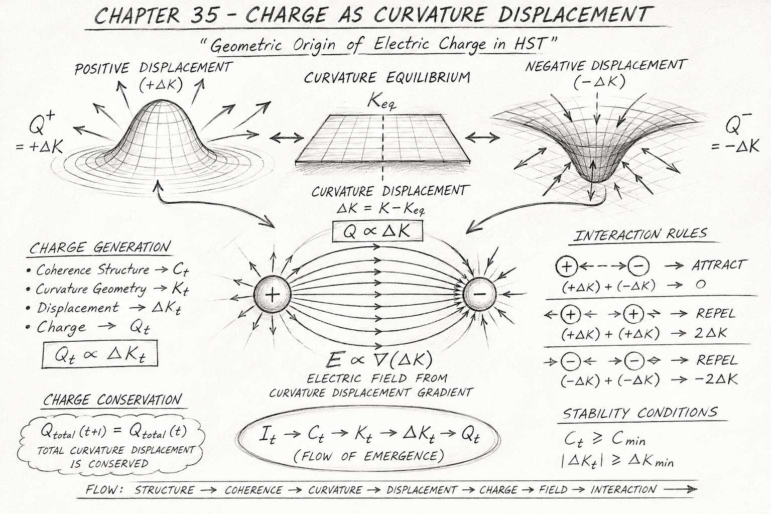
Figure 35.1 — Charge as Curvature Displacement in Holographic Space-Time

The diagram illustrates the HST interpretation of electric charge as a geometric consequence of curvature displacement within a coherence field. Rather than treating charge as an intrinsic property attached to particles, the figure shows how charge emerges naturally when local curvature deviates from an equilibrium configuration.

The diagram is organised as a complete causal sequence beginning with curvature equilibrium, progressing through displacement formation, charge generation, field emergence, interaction behaviour, conservation laws, and finally system evolution.

1. Curvature Equilibrium

The upper-left panel establishes the reference state of the system.

\[ K_{\mathrm{eq}} \]

is represented as a flat geometric surface corresponding to a balanced coherence configuration.

In this state:\Delta K = 0

\[ \Delta K = 0 \]

and therefore:

\[ Q = 0 \]

No net charge exists because no curvature displacement exists.

This equilibrium geometry acts as the baseline from which all charge states are measured.

Within HST, neutrality is therefore not a separate physical substance but simply the absence of displacement from geometric balance.

2. Curvature Displacement

The second panel introduces deformation of the equilibrium geometry.

The diagram illustrates curvature becoming displaced relative to the equilibrium surface.

This displacement is quantified as:

\[ \Delta K = K - K_{\mathrm{eq}} \]

where:

  • KK is the observed curvature state,
  • KeqK_{eq} is the equilibrium curvature.

The diagram emphasizes that charge originates from deviation rather than from an independently existing quantity.

The larger the displacement from equilibrium, the larger the resulting charge magnitude.

Telephone:
01377 236594

3. Charge Definition

The central charge-definition panel formalises the relationship:

\[ Q \propto \Delta K \]

This equation represents the core hypothesis of Chapter 35.

Charge becomes a direct measure of curvature displacement.

The figure identifies three possible states:

Positive Charge

\[ \Delta K > \epsilon \]

A positive displacement orientation generates:

\[ Q = + \]

Negative Charge

\[ \Delta K < -\epsilon \]

An opposite displacement orientation generates:

\[ Q = - \]

Neutral State

\[ \left| \Delta K \right| \leq \epsilon \]

The geometry remains sufficiently close to equilibrium and no net charge appears.

The neutrality threshold ε\varepsilon prevents microscopic fluctuations from being interpreted as stable charge states.

4. Curvature Displacement States

The large central illustrations depict the three geometric charge configurations.

Positive Displacement

The upward curvature deformation represents:

\[ Q^{+} = +\Delta K \]

The outward-directed arrows indicate a positive displacement orientation.

Equilibrium

The flat geometry represents:

\[ Q = 0 \]

No displacement exists.

Negative Displacement

The inward curvature depression represents:

\[ Q^{-} = -\Delta K \]

The inward-directed arrows indicate negative displacement orientation.

The symmetry of the diagrams highlights that positive and negative charge are mirror-image geometric states.

5. Electric Field Generation

The upper-right panel shows how charge generates electromagnetic structure.

The flow defines:

\[ E \propto \nabla(\Delta K) \]

meaning electric fields arise from spatial gradients of curvature displacement.

The field-line illustration between positive and negative charges represents the geometric transition between opposing displacement states.

Within HST:

  • Charge corresponds to displacement.
  • Electric fields correspond to displacement gradients.

The field is therefore not fundamental but emerges from the geometry of displacement itself.

6. Interaction Between Charges

The interaction panel demonstrates how attraction and repulsion emerge naturally from curvature geometry.

Opposite Charges

\[ (+\Delta K) + (-\Delta K) \]

When opposite displacement orientations interact, the curvature imbalance decreases.

The figure shows displacement cancellation.

This produces:

  • Reduced coherence tension
  • Lower geometric stress
  • Attraction

Symbolically:

\[ (+\Delta K) + (-\Delta K) \rightarrow 0 \]

The system evolves toward equilibrium.

Like Charges

The right-hand illustration shows identical displacement orientations interacting.

For example:

\[ (+\Delta K) + (+\Delta K) \]

The displacement magnitude increases.

Curvature imbalance grows.

Coherence tension rises.

The field responds by driving the structures apart.

This produces repulsion.

Similarly:

\[ (-\Delta K) + (-\Delta K) \]

also increases imbalance and produces repulsion.

Thus both attraction and repulsion emerge from the same geometric principle.

7. Stability Conditions

The lower centre panel introduces the requirements for persistent charge structures.

Coherence Stability

\[ C \geq C_{\min} \]

The system must possess sufficient coherence to maintain a stable displacement.

Without adequate coherence the charge state collapses.


Displacement Stability

\[ \left| \Delta K \right| \geq \Delta K_{\min} \]

Displacement must exceed a minimum threshold before it becomes physically meaningful.

Small fluctuations are treated as transient noise.


Field Continuity

\[ \nabla \cdot \mathbf{E} = \frac{\rho}{\varepsilon_0} \]

The field structure must remain continuous throughout evolution.

This requirement ensures stable electromagnetic behaviour.

8. Charge Conservation

The right-hand conservation panel introduces one of the strongest invariants of the model:

\[ Q_{\mathrm{total}}(t+1) = Q_{\mathrm{total}}(t) \]

The diagram emphasises that total curvature displacement remains conserved.

Charge may:

  • Move through the field
  • Redistribute
  • Separate
  • Recombine

but cannot appear or disappear spontaneously.

This conservation law emerges from geometric continuity within the coherence field.

9. System Evolution

The final panel shows recursive state progression:

\[ S_t \rightarrow S_{t+1} \]

Interactions modify:

  • Coherence geometry
  • Curvature distribution
  • Charge structure
  • Field configuration

This reflects the recursive evolution principle used throughout HST.

Reality is represented as a continuously updating coherence network rather than a static collection of particles.

Telephone:
01377 236594

10. Flow Sequence Summary

The bottom flow sequence condenses the entire chapter into a single emergence pathway:

\[ I_t \rightarrow C_t \rightarrow K_t \rightarrow \Delta K_t \rightarrow Q_t \rightarrow E_t \rightarrow R_t \rightarrow S_{t+1} \]

where:

Stage Meaning
I_t Physical structure
C_t Coherence map
K_t Curvature geometry
ΔK_t Curvature displacement
Q_t Charge state
E_t Electric field
R_t Interaction response
S_t+1 Updated system state

Scientific Interpretation

The figure presents a complete HST reformulation of electric charge.

Rather than beginning with charge as a fundamental particle property, the diagram derives charge from curvature displacement within a coherence field.

The overall causal chain becomes:

Structure→Coherence→
Curvature→
Displacement→
Charge→Field→Interaction→
Evolution

Under this interpretation, positive and negative charge become opposite geometric orientations, electric fields become displacement gradients, attraction becomes curvature cancellation, repulsion becomes curvature reinforcement, and charge conservation becomes a direct consequence of geometric continuity.

The diagram therefore provides the complete visual representation of Charge as Curvature Displacement within the Holographic Space-Time framework

Diagram → Flow Mapping Table

Diagram Element Diagram Location Flow Algebra Representation
Equilibrium Surface Panel 1 – Curvature Equilibrium K_eq
Flat Geometry Central equilibrium grid ΔK_t = 0
Neutral State Equilibrium configuration Q_t = 0
Curvature Deformation Panel 2 – Curvature Displacement ΔK_t = K_t - K_eq
Upward Curvature Dome Positive displacement illustration ΔK_t > 0
Downward Curvature Well Negative displacement illustration ΔK_t < 0
Positive Charge Region Positive displacement state Q_t = +ΔK_t
Negative Charge Region Negative displacement state Q_t = -ΔK_t
Neutral Threshold Zone Charge definition panel |ΔK_t| ≤ ε
Charge Formation Box Panel 3 – Charge Definition Q_t ∝ ΔK_t
Physical Structure Layer Flow sequence summary I_t
Coherence Mapping Layer Flow sequence summary C_t = CoherenceMap(I_t)
Curvature Layer Flow sequence summary K_t = Curvature(C_t)
Displacement Layer Flow sequence summary ΔK_t = K_t - K_eq
Charge Layer Flow sequence summary Q_t
Electric Field Layer Flow sequence summary E_t
Interaction Layer Flow sequence summary R_t
Next State Layer Flow sequence summary S_t+1
Electric Field Lines Panel 4 – Electric Field Generation E_t ∝ ∇(ΔK_t)
Field Gradient Arrows Between positive and negative charges ∇(ΔK_t)
Field Continuity Electric field panel E_t ≠ ∅
Positive Charge Symbol Positive displacement geometry Q+
Negative Charge Symbol Negative displacement geometry Q−
Opposite-Charge Pair Interaction panel (left) Q_aQ_b < 0
Attraction Arrows Opposite-charge interaction R_t = Attraction
Curvature Cancellation Opposite-charge interaction (+ΔK)+(-ΔK) → 0
Reduced Tension State Opposite-charge interaction T_t ↓
Like-Charge Pair (+,+) Interaction panel (right) Q_aQ_b > 0
Like-Charge Pair (-,-) Interaction panel (right) Q_aQ_b > 0
Repulsion Arrows Like-charge interaction R_t = Repulsion
Curvature Reinforcement Like-charge interaction (+ΔK)+(+ΔK) → 2ΔK
Negative Reinforcement Like-charge interaction (−ΔK)+(−ΔK) → −2ΔK
Increased Tension State Repulsion configuration T_t ↑
Coherence Stability Box Stability Conditions panel C_t ≥ C_min
Stable Displacement Requirement Stability Conditions panel |ΔK_t| ≥ ΔK_min
Field Stability Requirement Stability Conditions panel E_t = Continuous
Charge Conservation Box Panel 6 – Charge Conservation Q_total(t+1)=Q_total(t)
Conserved Displacement Statement Charge conservation panel dQ_total/dt = 0
Curvature Continuity Charge conservation panel ΔK_total(t+1)=ΔK_total(t)
System Evolution Arrow Panel 8 – System Evolution S_t → S_t+1
Recursive Update Process Final evolution stage Execution(S_t) → S_t+1
Complete Emergence Pathway Bottom summary flow I_t → C_t → K_t → ΔK_t → Q_t → E_t → R_t → S_t+1
HST Charge Principle Entire diagram Q_t ∝ (K_t - K_eq)
HST Electric Field Principle Entire diagram E_t ∝ ∇(K_t - K_eq)
HST Attraction Principle Interaction subsystem Curvature cancellation minimises imbalance
HST Repulsion Principle Interaction subsystem Curvature reinforcement increases imbalance
HST Conservation Principle Conservation subsystem Total curvature displacement remains invariant
HST Stability Principle Stability subsystem Stable charge requires coherence and displacement thresholds
Full Chapter Representation Entire figure Charge emerges from curvature displacement within a coherent geometric field

Execution Guarantee Statement

Chapter 35 — Charge as Curvature Displacement

Purpose

The Charge as Curvature Displacement flow is constructed to guarantee the emergence, persistence, interaction, and conservation of electric charge from geometric curvature displacement within a coherent field structure.

The flow does not assume charge as a fundamental property. Instead, charge is generated directly from measurable displacement relative to a curvature equilibrium state and remains stable only while coherence, displacement continuity, and conservation constraints are maintained.

Structural Guarantee

The flow guarantees that every observable charge state originates from an underlying curvature displacement:

\[ \Delta K_t = K_t - K_{\mathrm{eq}} \]

and therefore:

\[ Q_t \propto \Delta K_t \]

No charge state can emerge without a corresponding geometric displacement.

This prevents arbitrary charge creation and ensures that charge remains structurally tied to the curvature configuration of the coherence field.

Positive and Negative Charge Guarantee

The flow guarantees that charge polarity emerges directly from displacement orientation.

Positive charge is generated whenever:

\[ \Delta K_t > \epsilon \]

Negative charge is generated whenever:

\[ \Delta K_t < -\epsilon \]

Neutrality occurs whenever:

\[ \left| \Delta K_t \right| \leq \epsilon \]

Because polarity is determined entirely by displacement direction, positive and negative charge remain symmetric geometric solutions of the same underlying system.

Electric Field Guarantee

The flow guarantees that every stable charge configuration produces an associated electric field through spatial displacement gradients.

\[ E_t \propto \nabla(\Delta K_t) \]

If curvature displacement exists, then field generation follows automatically.

Consequently:

  • Larger displacement gradients generate stronger fields.
  • Smaller displacement gradients generate weaker fields.
  • Zero displacement gradient produces no field.

The existence of charge therefore guarantees the existence of an electromagnetic field structure.

Interaction Guarantee

The flow guarantees deterministic interaction behaviour between charged structures.

For opposite displacement orientations:

\[ (+\Delta K) + (-\Delta K) \rightarrow 0 \]

the system reduces curvature imbalance and generates attraction.

For identical displacement orientations:

\[ (+\Delta K) + (+\Delta K) \rightarrow 2\Delta K \]

or

\[ (-\Delta K) + (-\Delta K) \rightarrow -2\Delta K \]

the system increases curvature imbalance and generates repulsion.

Thus attraction and repulsion are guaranteed outcomes of displacement geometry rather than externally imposed force rules.

Conservation Guarantee

The flow guarantees conservation of total charge through conservation of total curvature displacement.Q_{total}(t+1) = Q_{total}(t)

\[ Q_{\mathrm{total}}(t+1) = Q_{\mathrm{total}}(t) \]

At every recursive update:

\[ S_t \rightarrow S_{t+1} \]

charge may:

  • Transfer,
  • Redistribute,
  • Separate,
  • Recombine,Transfer,
  • Redistribute,
  • Separate,
  • Recombine,

but total displacement remains invariant.

The flow therefore prohibits spontaneous creation or destruction of net charge.

Stability Guarantee

A charge state is guaranteed to remain stable only when the following conditions hold:

Coherence Stability

\[ C_t \geq C_{\min} \]

Displacement Stability

\[ \left| \Delta K_t \right| \geq \Delta K_{\min} \]

Field Continuity

\[ E_t \neq \emptyset \]

Conservation Validity

\[ Q_{\mathrm{total}}(t+1) = Q_{\mathrm{total}}(t) \]

When all conditions are satisfied, the charge configuration persists across recursive system updates.

Failure Guarantee

The flow guarantees deformation or collapse whenever any stability condition is violated.

Failure occurs when:

\[ C_t < C_{\min} \]

or

\[ \left| \Delta K_t \right| < \Delta K_{\min} \]

or

\[ Q_{\mathrm{total}}(t+1) \neq Q_{\mathrm{total}}(t) \]

or field continuity becomes disrupted.

Under these circumstances:

\[ \mathrm{Execution}(S_t) = \mathrm{FAIL\_OR\_DEFORM} \]

indicating loss of stable charge structure.

Recursive Evolution Guarantee

The flow guarantees that charge remains embedded within the broader recursive evolution of the coherence field.

The complete execution pathway remains:

\[ I_t \rightarrow C_t \rightarrow K_t \rightarrow \Delta K_t \rightarrow Q_t \rightarrow E_t \rightarrow R_t \rightarrow S_{t+1} \]

Each stage is causally generated from the previous stage.

No independent charge variable is inserted externally.

Every electromagnetic phenomenon emerges from the underlying curvature geometry.

Formal Execution Guarantee

\[ (C_t \geq C_{\min}) \;\wedge\; \left( \left| \Delta K_t \right| \geq \Delta K_{\min} \right) \;\wedge\; \left( Q_{\mathrm{total}}(t+1) = Q_{\mathrm{total}}(t) \right) \;\wedge\; (E_t \neq \emptyset) \]

⟹

\[ \mathrm{Execution}(S_t) = \mathrm{STABLE} \]


Guarantee Statement

If coherence remains above the minimum stability threshold, curvature displacement remains continuous, total displacement is conserved, and field gradients remain well-defined, then charge will persist as a stable geometric property of the coherence field.

Positive and negative charge will emerge as opposite displacement orientations, electric fields will arise from displacement gradients, attraction and repulsion will emerge from curvature balancing dynamics, and the system will evolve recursively while preserving global charge conservation.
Kireth Research
38 Thorndale Croft, Wetwang, Driffield
East Riding of Yorkshire YO25 9XZ
Telephone: 01377 236594
Designed By