The Casimir Effect

Author: Mark Higgins
© Mark Anthony Higgins 11 October 2025

Revised Date: 18th June 2026

Audio Overview

Introduction

The Casimir Effect is one of the most remarkable and experimentally verified phenomena in quantum physics. First predicted by Dutch physicist Hendrik Casimir in 1948, the effect demonstrates that two uncharged conductive plates placed extremely close together in a vacuum experience a measurable attractive force.

Within conventional quantum field theory, this force is explained as arising from vacuum fluctuations: the continuous creation and annihilation of virtual particles throughout empty space. The presence of the plates restricts which vacuum modes can exist between them, producing an imbalance in vacuum energy that pushes the plates together.

The Casimir Effect is often regarded as one of the strongest experimental indications that the vacuum is not truly empty.

Within Holographic Space-Time (HST), however, the phenomenon can be reinterpreted without requiring an infinite sea of virtual particles. Instead, the effect emerges naturally from boundary coherence geometry and the suppression of allowable field configurations.

1. The Traditional Interpretation

In standard quantum mechanics and quantum field theory, empty space contains fluctuating electromagnetic fields at every frequency.

The vacuum is therefore described as possessing a non-zero ground-state energy.

For every allowable mode:

\[ E = \frac{1}{2} \hbar \omega \]

where:

  • EE is vacuum mode energy
  • ℏ\hbar is the reduced Planck constant
  • ω\omega is angular frequency

Because an infinite number of modes exist, the vacuum contains an enormous amount of theoretical energy.

When two conducting plates are brought close together:

  • Some wavelengths fit between the plates.
  • Others do not.
  • The spectrum of allowed modes becomes restricted.

Outside the plates:

  • More modes remain available.

Inside the plates:

  • Fewer modes can exist.

The imbalance produces a net inward force.

2. The Conceptual Difficulty

Although experimentally successful, the traditional explanation raises several conceptual challenges:

Infinite Vacuum Energy

The vacuum energy calculation initially diverges toward infinity.

Large mathematical cancellations are required to recover finite results.

Virtual Particle Interpretation

The notion of virtual particles is often used heuristically rather than as directly observable entities.

Dependence on Boundary Conditions

The force appears only when boundaries are introduced.

This suggests the phenomenon may be fundamentally geometric rather than particle-based.

These observations motivate a boundary-centered reinterpretation.

3. The HST Reinterpretation

Within HST:

Space is not an empty container filled with fluctuating particles.

Instead:

Space emerges from a structured coherence field encoded across boundaries.  Field behaviour is determined by permissible coherence configurations.

The vacuum is therefore:

The lowest-energy coherent boundary state.

Rather than asking:

"What particles exist in the vacuum?"

HST asks:

"What coherence modes are permitted by the surrounding boundary geometry?"

The Casimir force then becomes a direct consequence of boundary mode suppression.

4. Boundary Mode Suppression

Consider two parallel conducting plates.

The plates impose strict coherence constraints on the field.

Only certain standing coherence modes can exist between them.

Many larger-scale configurations become forbidden.

This creates:

\[ N_{\mathrm{inside}} < N_{\mathrm{outside}} \]

where:

  • NinsideN_{\text{inside}} = allowable coherence modes between plates
  • NoutsideN_{\text{outside}} = allowable coherence modes outside plates

The result is a coherence density imbalance.

5. Coherence Pressure

HST treats field configurations as structured coherence pathways.

A region supporting more allowable configurations possesses greater coherence freedom.

A region supporting fewer configurations possesses greater coherence restriction.

The field naturally evolves toward reducing this asymmetry.

This produces an effective pressure:

\[ P_C \propto \Delta M \]

where:

  • PCP_C = Casimir pressure
  • ΔM\Delta M = difference in allowable coherence modes

The plates move together because the surrounding coherence geometry seeks a lower-tension configuration.

6. Geometric Interpretation

Under HST, the Casimir Effect is not a force generated by particles.

It is a geometric response of the coherence field to constrained boundaries.

The sequence becomes:

Step 1

Boundaries are introduced.

Step 2

Allowable coherence modes become restricted.

Step 3

Coherence density becomes asymmetric.

Step 4

Field tension develops.

Step 5

The geometry relaxes toward a lower-energy configuration.

Step 6

The plates move together.

The observed force emerges naturally from coherence minimisation.

7. Why the Effect Increases at Small Distances

As plate separation decreases:

  • More coherence modes are excluded.
  • Internal configuration space shrinks.
  • Boundary restrictions intensify.

Thus:

\[ \Delta M \uparrow \]

and therefore:

\[ P_C \uparrow \]

The rapidly increasing attraction at nanometre scales follows directly from increasing geometric confinement.

Telephone:
01377 236594

8. Casimir Effect as Evidence for Boundary Physics

One of the most important implications of the Casimir Effect is that measurable forces can emerge purely from boundary constraints.

  • No charge is required.
  • No mass is required.
  • No classical field source is required.
  • Only geometry and boundary conditions are needed.

This observation aligns closely with the central HST principle:

Physical phenomena emerge from the structure of allowable boundary configurations rather than from objects existing independently within space.

The Casimir Effect therefore becomes a direct experimental example of boundary-driven reality.

9. Relationship to Other HST Phenomena

The same mechanism appears throughout HST.

Quantum Tunnelling

Boundary restrictions alter allowable transition pathways.

Entanglement

Shared boundary structures create correlated coherence maps.

Dark Matter

Residual coherence gradients emerge from large-scale boundary encoding.

Gravity

Mass corresponds to persistent coherence density gradients.

Casimir Effect

Boundary constraints suppress allowable field modes and generate measurable curvature pressure.

All arise from the same underlying principle:

Geometry→Mode Restriction→Coherence Gradient→Observable Phenomenon

10. Scientific Significance

The Casimir Effect demonstrates that physical reality responds to information about boundaries.

Within conventional physics this appears as vacuum-energy imbalance.

Within HST it appears as coherence-mode suppression.

Both descriptions predict the same measurable force.

However, the HST interpretation replaces virtual-particle intuition with a geometric framework based on boundary coherence.

In this view, the Casimir Effect is not evidence that empty space contains an infinite sea of particles. Instead, it is evidence that the structure of permissible field configurations possesses physical reality and that boundaries actively shape the geometry from which forces emerge.

Conclusion

The Casimir Effect provides one of the clearest demonstrations that boundaries possess physical significance. While conventional quantum theory explains the phenomenon through vacuum fluctuations and virtual particles, HST reformulates it as a consequence of boundary-induced coherence suppression.

When conductive plates constrain the allowable field configurations of space, a coherence imbalance forms between the interior and exterior regions. The field then relaxes toward a lower-tension state, producing the observed attraction.

Within HST, the Casimir force is therefore not a mysterious vacuum phenomenon but a natural consequence of boundary geometry, coherence restriction, and the tendency of structured systems to minimise informational tension. It stands as a powerful example of how measurable physical forces can emerge directly from the organisation of allowable boundary states.

Flow: CasimirEffect_BoundaryModeSuppression
Version: 1.0
Authors:
  - Mark Higgins
  - Sky

Domain: Quantum_Field_Geometry
Framework: Holographic_Space_Time

Purpose:
  To model the Casimir Effect as boundary-induced suppression of allowable
  coherence modes, producing a measurable pressure imbalance between constrained
  and unconstrained regions of space.

Inputs:
  Plates:
    Geometry: Parallel_Conductive_Boundaries
    Separation: d
    Surface_State: Conductive
    Boundary_Condition: Mode_Restriction

  Field:
    Vacuum_State: Coherent_Ground_State
    Mode_Set: M
    External_Modes: M_outside
    Internal_Modes: M_inside

  Constants:
    hbar: Reduced_Planck_Constant
    c: Speed_Of_Light
    C_min: Minimum_Coherence_Threshold
    epsilon: Stability_Tolerance

States:
  B_t:
    description: Boundary geometry at time t

  M_inside_t:
    description: Allowed coherence modes between the plates

  M_outside_t:
    description: Allowed coherence modes outside the plates

  Delta_M_t:
    description: Mode imbalance across the plate boundary

  rho_C_t:
    description: Coherence density distribution

  P_C_t:
    description: Coherence pressure generated by mode imbalance

  F_C_t:
    description: Effective Casimir force

Process:
  Initialise:
    B_t := Define_Boundaries(Plates)
    M_outside_t := All_Allowed_Vacuum_Modes(Field)
    M_inside_t := Apply_Boundary_Restrictions(M_outside_t, B_t, d)

  Mode_Suppression:
    Delta_M_t := M_outside_t - M_inside_t

  Coherence_Density_Update:
    rho_C_t := Map_Mode_Density(M_inside_t, M_outside_t)

  Pressure_Generation:
    P_C_t := Pressure_From_Mode_Imbalance(Delta_M_t, d)

  Force_Output:
    F_C_t := Integrate_Pressure_Over_Surface(P_C_t, Plates)

Equations:
  Vacuum_Mode_Energy:
    E_mode = 1/2 * hbar * omega

  Mode_Inequality:
    N_inside < N_outside

  Mode_Imbalance:
    Delta_M = N_outside - N_inside

  Coherence_Pressure:
    P_C proportional_to Delta_M

  Distance_Dependence:
    Delta_M increases_as d decreases

  Force_Direction:
    F_C points_toward Reduced_Separation

HST_Reinterpretation:
  Standard_Model_View:
    Casimir_Effect := Vacuum_Fluctuation_Energy_Imbalance

  HST_View:
    Casimir_Effect := Boundary_Coherence_Mode_Suppression

  Meaning:
    The plates do not attract because empty space contains physical particles
    pushing from outside. They move together because the boundary geometry
    restricts allowable coherence states between them, creating an asymmetric
    field-tension condition.

Execution_Path:
  B_t
    -> Boundary_Restriction
    -> M_inside_t
    -> Delta_M_t
    -> rho_C_t
    -> P_C_t
    -> F_C_t
    -> Plate_Motion

Validity_Conditions:
  - d > 0
  - Plates_are_parallel == true
  - Boundary_Condition == Conductive_Mode_Restriction
  - N_inside < N_outside
  - rho_C_t >= C_min
  - abs(Field_Instability) <= epsilon

Failure_Conditions:
  - d <= 0
  - Plates_are_parallel == false
  - Boundary_Condition == None
  - N_inside >= N_outside
  - rho_C_t < C_min

Outputs:
  Casimir_Pressure: P_C_t
  Casimir_Force: F_C_t
  Boundary_Mode_Suppression: Delta_M_t
  Coherence_Density_Map: rho_C_t
  Execution_Result: Boundary_Attraction

Conclusion:
  The Casimir Effect is executed as a boundary-coherence phenomenon.
  Conductive plates restrict the internal set of allowable field modes.
  This produces a coherence-density imbalance between interior and exterior
  regions, generating pressure toward reduced separation.
  In HST, the observed force is not caused by virtual particles as objects,
  but by geometric suppression of permissible boundary states.

What This Flow Implements

Introduction

The CasimirEffect_BoundaryModeSuppression flow implements a complete Holographic Space-Time (HST) description of the Casimir Effect as a consequence of boundary-induced coherence restriction rather than as a direct manifestation of virtual particle interactions.

The flow models how conductive boundaries alter the set of allowable field configurations within a region of space, producing measurable pressure gradients that drive physical motion. Rather than treating the vacuum as an infinite sea of fluctuating particles, the flow treats the vacuum as a structured coherence field whose behaviour is determined by geometric constraints imposed upon it.

The implementation provides a deterministic sequence linking boundary geometry to force generation through mode suppression, coherence-density redistribution, and tension minimisation.

1. Representation of Physical Boundaries

The first function of the flow is to establish the physical geometry responsible for the phenomenon.

The conductive plates are represented as:

\[ B_t \]

where:

  • BtB_t denotes the active boundary configuration at time tt
  • The boundaries define permissible field conditions
  • The geometry determines which coherence structures may exist

Within the implementation, the plates are not treated as force sources.

Instead, they act as information constraints that modify the allowable state space of the surrounding coherence field.

This distinction is fundamental to the HST interpretation.

The boundaries shape reality rather than generate force directly.

2. Construction of the Available Mode Space

The flow next constructs the complete set of possible vacuum modes:

\[ M_{\mathrm{outside}} \]

representing the unrestricted field configuration space.

This state corresponds to the maximum allowable coherence freedom available in the surrounding vacuum.

The flow assumes that empty space supports a large set of possible field structures whose existence depends on geometric compatibility.

The unrestricted region therefore serves as the reference state against which the constrained region is measured.

Telephone:
01377 236594

3. Boundary-Induced Mode Suppression

The central operation of the flow is the application of boundary constraints.

This occurs through:

Minside​=ApplyBoundaryRestrictions(Moutside​,Bt​,d)

where:

  • dd is plate separation
  • MinsideM_{\text{inside}} represents modes surviving the restriction process

Only modes compatible with the boundary geometry remain.

Modes that cannot satisfy the imposed conditions are removed from the allowable state space.

The flow therefore implements a direct reduction in informational freedom.

This is the mechanism responsible for the emergence of the Casimir effect.

4. Measurement of Mode Imbalance

Once the internal mode set has been established, the flow calculates the asymmetry:

\[ \Delta M = N_{\mathrm{outside}} - N_{\mathrm{inside}} \]

This quantity measures how strongly the plates distort the local coherence landscape.

Physically:

  • Large separations produce small imbalances.
  • Small separations produce large imbalances.

The flow therefore creates a direct quantitative link between geometry and observable force.

The imbalance is not interpreted as missing particles.

It is interpreted as missing permissible field configurations.

5. Construction of the Coherence Density Map

The next stage transforms mode imbalance into a spatial structure.

The flow generates:

\[ \rho_C \]

representing coherence density.

This field describes how informational freedom is distributed throughout the surrounding geometry.

Regions supporting many allowable configurations possess higher coherence freedom.

Regions supporting fewer allowable configurations possess greater restriction.

The coherence density map therefore acts as the geometric equivalent of a pressure field.

6. Emergence of Coherence Pressure

The flow then converts coherence asymmetry into measurable pressure:

\[ P_C \propto \Delta M \]

This pressure is not a conventional mechanical pressure.

Instead, it represents a tendency of the coherence field to minimise restrictions and reduce geometric tension.

The implementation assumes that field configurations naturally evolve toward lower-tension states.

This is the same coherence-minimisation principle used throughout HST to explain:

  • Gravity
  • Entropy
  • Field evolution
  • Quantum transitions
  • Information flow

The Casimir Effect becomes another manifestation of the same underlying law.

7. Force Generation

The pressure field is integrated across the conductive surfaces:

\[ F_C = \int P_C \, dA \]

where:

  • FCF_C is the Casimir force
  • AA is plate area

This stage converts distributed geometric tension into observable mechanical motion.

The force is not inserted into the model.

It emerges from the preceding coherence calculations.

This is a critical feature of the flow.

Physical attraction is produced rather than assumed.

8. Dynamic Dependence on Plate Separation

The implementation explicitly captures the experimentally observed increase in force at small separations.

As:

\[ d \downarrow \]

the number of allowable internal modes decreases:

\[ N_{\mathrm{inside}} \downarrow \]

which produces:

\[ \Delta M \uparrow \]

leading to:

\[ P_C \uparrow \]

and therefore:

\[ F_C \uparrow \]

The flow naturally reproduces the increasing attraction measured in laboratory experiments.

No additional assumptions are required.

9. Replacement of the Virtual Particle Interpretation

One of the most significant functions of the flow is conceptual.

Traditional descriptions often explain the Casimir Effect using virtual particles.

The flow replaces this picture entirely.

Instead of:

\[ \mathrm{Virtual\ Particles} \rightarrow \mathrm{Force} \]

the implementation uses:

Boundary Geometry→Mode Restriction→Coherence Gradient→Pressure→Force

This transformation shifts the explanation from particle ontology to geometric information structure.

The experimentally observable predictions remain unchanged.

The interpretation becomes structurally simpler and more unified with the rest of HST.

10. Integration into the HST Framework

The flow is designed to operate as part of a larger coherence-based physical architecture.

The same mechanism appears elsewhere in HST:

Diagram Object Flow Symbol HST Meaning
Fibre B_t Boundary geometry
Core n_core High-coherence channel
Cladding n_cladding Confinement region
Coherence Field C_t Internal propagation map
Density ρ_C Stability field
Gradient ∇ρ_C Guidance direction
Alignment R_t Local propagation vector
Transfer x_t+1 Microscopic motion
Segment Path_local Flat propagation element
Reconstruction Path_global Emergent fibre path
Curvature K_app Observer-inferred bending
Stable Fibre Execution(P_t)=GUIDED_PROPAGATION Successful coherence transport
HST Result Path_local ≈ Flat → Path_global ≈ Curved Apparent curvature emerges from accumulated local transfers

This allows the Casimir Effect to be incorporated into a single geometric framework rather than existing as a specialised quantum anomaly.

11. Scientific Significance of the Flow

The flow implements a complete causal chain linking:

Boundary Structure→Allowed Modes→Coherence Density→Pressure→Force

Every stage remains physically interpretable.

Every stage corresponds to measurable consequences.

Most importantly, the implementation demonstrates that a measurable force can emerge solely from restrictions imposed on allowable field configurations.

  • No charge is required.
  • No mass is required.
  • No classical force source is required.

Only boundary geometry and coherence structure are necessary.

Conclusion

The CasimirEffect_BoundaryModeSuppression flow implements a fully geometric HST reformulation of the Casimir Effect. It begins with conductive boundary conditions, calculates the suppression of allowable coherence modes, constructs the resulting coherence-density imbalance, generates a pressure field from that imbalance, and integrates the pressure into an observable attractive force.

Within this framework, the Casimir Effect is not treated as evidence for a vacuum filled with virtual particles, but as a direct manifestation of boundary-controlled coherence geometry. The flow therefore provides a unified, deterministic, and structurally consistent explanation that connects quantum vacuum phenomena to the broader HST principles of boundary encoding, coherence minimisation, and emergent physical behaviour.

How to Read This Flow

Introduction

The CasimirEffect_BoundaryModeSuppression flow describes how the Casimir Effect emerges from restrictions imposed upon allowable coherence configurations by conductive boundaries.

Unlike traditional mathematical derivations that begin with vacuum-energy calculations, this flow begins with geometry. The reader follows the transformation of a physical boundary configuration into a measurable force through a sequence of coherence-based operations.

The flow should be read from top to bottom, with each section representing a progressively deeper level of physical organisation.

At every stage the flow answers a specific scientific question:

  • 1. What boundaries exist?
  • 2. What field configurations are allowed?
  • 3. How do those configurations differ between regions?
  • 4. How does that difference create a gradient?
  • 5. How does the gradient generate pressure?
  • 6. How does pressure become force?

The complete chain explains the observed attraction between closely spaced conductive plates.

1. Begin with the Flow Header

The opening section identifies the physical phenomenon being modelled.

Flow: CasimirEffect_BoundaryModeSuppression
Version: 1.0
Domain: Quantum_Field_Geometry
Framework: Holographic_Space_Time

This tells us:

  • The system concerns the Casimir Effect.
  • The mechanism involves suppression of field modes.
  • The model operates within HST.
  • The explanation is geometric rather than particle-based.

Before reading further, understand that the flow treats the vacuum as a coherence field whose behaviour depends upon boundary conditions.

2. Read the Purpose Statement

The purpose defines the scientific objective.

Purpose:
  To model the Casimir Effect as boundary-induced suppression
  of allowable coherence modes.

This statement establishes the central hypothesis:
The force arises because boundaries alter what field configurations are permitted.

The remainder of the flow explains how this happens.

Telephone:
01377 236594

3. Examine the Inputs

The inputs define the physical system.

Inputs:
  Plates
  Field
  Constants

These inputs represent the experimental setup.

Plates
Geometry: Parallel_Conductive_Boundaries
Separation: d

These define the physical boundaries.

The separation distance dd will later determine how many modes survive between the plates.

Field
Vacuum_State: Coherent_Ground_State
Mode_Set: M

The vacuum is represented as a collection of possible coherence structures.

The field contains many allowable configurations.

The boundaries will restrict these possibilities.

Constants
hbar
c
C_min
epsilon

These establish physical scales and numerical stability requirements.

4. Study the State Definitions

The next section introduces the variables that evolve throughout the flow.

Boundary State
B_t

Represents the active geometry.

This is the source of all later effects.

No boundary means no Casimir Effect.

Internal Modes
M_inside_t

These are the allowable field configurations that survive inside the plate gap.

This quantity becomes smaller as plate separation decreases.

External Modes
M_outside_t

Represents the unrestricted field outside the plates.

This acts as the reference state.

Mode Imbalance
Delta_M_t

Measures the difference between internal and external mode populations.

This quantity drives the entire phenomenon.

Coherence Density
rho_C_t

Represents how coherence freedom is distributed throughout space.

This is analogous to a pressure landscape.

Coherence Pressure
P_C_t

Represents the tension created by unequal coherence freedom.

This is the precursor to force generation.

Casimir Force
F_C_t

The observable outcome.

This is the measurable attraction seen experimentally.

Telephone:
01377 236594

5. Follow the Initialise Stage

The flow begins by constructing the geometry.

B_t := Define_Boundaries(Plates)

This creates the conductive boundaries.

Next:

M_outside_t := All_Allowed_Vacuum_Modes(Field)

The unrestricted vacuum state is calculated.

Then:

M_inside_t :=
Apply_Boundary_Restrictions(...)

The boundaries remove incompatible modes.

This is the first major transformation in the flow.

6. Read the Mode Suppression Stage

The flow now computes:

Delta_M_t :=
M_outside_t - M_inside_t

This operation measures how strongly the boundaries distort the field.

Scientifically:

\[ \Delta M = N_{\mathrm{outside}} - N_{\mathrm{inside}} \]

A large value means many modes have been excluded.

A small value means the vacuum remains largely unrestricted.

The Casimir Effect emerges directly from this difference.

7. Read the Coherence Density Update

Next:

rho_C_t :=
Map_Mode_Density(...)

This converts raw mode counts into a spatial coherence field.

The question being answered is:

Where does informational freedom exist?

Regions supporting many modes possess higher coherence freedom.

Regions supporting fewer modes possess lower coherence freedom.

The resulting density field encodes the asymmetry created by the plates.

8. Read the Pressure Generation Stage

The next operation computes:

P_C_t :=
Pressure_From_Mode_Imbalance(...)

This stage transforms geometry into dynamics.

Mathematically:

\[ P_C \propto \Delta M \]

The larger the mode imbalance, the larger the pressure.

The pressure represents the tendency of the coherence field to reduce restriction.

This is the driving mechanism of the effect.

9. Read the Force Output Stage

The pressure field is converted into force:

F_C_t :=
Integrate_Pressure_Over_Surface(...)

Equivalent to:

\[ F_C = \int P_C \, dA \]

The distributed pressure is accumulated across the plate surfaces.

The result is a measurable attraction.

The force is therefore an emergent property rather than a predefined input.

10. Interpret the Equations Section

The equations provide physical meaning for each stage.

Vacuum Mode Energy

\[ E_{\mathrm{mode}} = \frac{1}{2} \hbar \omega \]

Defines the energy associated with each allowable mode.


Mode Inequality

\[ N_{\mathrm{inside}} < N_{\mathrm{outside}} \]

Defines the essential requirement for the effect.


Mode Imbalance

\[ \Delta M = N_{\mathrm{outside}} - N_{\mathrm{inside}} \]

Measures suppression strength.


Pressure Relation

\[ P_C \propto \Delta M \]

Converts restriction into geometric tension.


Distance Dependence

\[ d \downarrow \Rightarrow \Delta M \uparrow \]

Explains why the force increases as the plates approach each other.

11. Study the HST Reinterpretation Block

This section contains the conceptual heart of the flow.

Traditional explanation:

Virtual Particles→Force

HST explanation:

Boundary Geometry→Mode Restriction→Coherence Gradient→Pressure→Force

This tells the reader how the phenomenon should be interpreted.

The physical predictions remain the same.

The causal mechanism changes.


12. Read the Execution Path Last

The execution path is the condensed summary of the entire model.

B_t
 -> Boundary_Restriction
 -> M_inside_t
 -> Delta_M_t
 -> rho_C_t
 -> P_C_t
 -> F_C_t
 -> Plate_Motion

This is the complete causal chain.

It can be read as:

  • Boundaries restrict allowable modes.
  • Mode restriction creates asymmetry.
  • Asymmetry creates coherence gradients.
  • Gradients generate pressure.
  • Pressure generates force.
  • Force moves the plates.

Everything in the flow exists to support this sequence.

Scientific Reading Summary

When reading this flow, follow the progression:

\[ B_t \rightarrow M_{\mathrm{inside}} \rightarrow \Delta M \rightarrow \rho_C \rightarrow P_C \rightarrow F_C \]

or, conceptually:

Boundary→Restriction→Imbalance→Density→Pressure→Force

Rather than viewing the vacuum as a sea of virtual particles, the reader should understand the flow as describing how geometry constrains permissible coherence structures, how those constraints create asymmetries in informational freedom, and how the resulting tension manifests as the experimentally observed Casimir attraction.

Flow → Equation Tri-Mapping Table

Flow Layer Equation Layer Physical Interpretation
B_t Boundary Conditions Conductive plates defining allowable field states
d Plate Separation Distance controlling mode suppression strength
M_outside N_outside Total allowable vacuum modes outside plates
M_inside N_inside Allowed vacuum modes between plates
Mode_Suppression N_inside < N_outside Internal configuration space is restricted
Delta_M ΔM = N_outside - N_inside Net mode imbalance created by boundaries
ρ_C ρ_C = f(ΔM) Coherence-density distribution generated by suppression
Gradient(ρ_C) ∇ρ_C Spatial coherence-density gradient
Pressure_Generation P_C ∝ ΔM Coherence pressure emerges from mode asymmetry
Pressure_Field P_C = f(∇ρ_C) Local pressure determined by coherence gradients
Surface_Integration F_C = ∫ P_C dA Pressure accumulated across plate area
Force_Output F_C > 0 Observable Casimir attraction
Distance_Reduction d ↓ Plates move closer together
Mode_Restriction_Increase d ↓ ⇒ N_inside ↓ Smaller separation removes additional modes
Imbalance_Growth N_inside ↓ ⇒ ΔM ↑ Suppression becomes stronger
Pressure_Growth ΔM ↑ ⇒ P_C ↑ Coherence pressure increases
Force_Growth P_C ↑ ⇒ F_C ↑ Attraction increases rapidly
Vacuum_Mode_Energy E_mode = ½ℏω Energy associated with each allowable mode
Stable_Coherence ρ_C ≥ C_min Minimum coherence threshold maintained
Execution(P_t) CASIMIR_ATTRACTION Successful boundary-force generation

Flow Compression Chain
B_t
→ M_inside
→ ΔM
→ ρC
→ ∇ρC
→ P_C
→ F_C
→ d↓

Equation Compression Chain
Ninside < Noutside
→ ΔM = Noutside − Ninside
→ ρC = f(ΔM)
→ ∇ρC
→ P_C ∝ ΔM
→ F_C = ∫P_C dA

HST Compression Chain
Boundary Geometry
→ Mode Restriction
→ Coherence Imbalance
→ Density Gradient
→ Coherence Pressure
→ Casimir Force

Standard Physics ⇄ HST Mapping

Standard Interpretation HST Interpretation
Vacuum Fluctuations Coherence Field Structure
Virtual Particles Allowed Boundary Modes
Vacuum Energy Difference Coherence Density Difference
Zero-Point Pressure Boundary Coherence Pressure
Attractive Force Tension Minimisation
Quantum Vacuum Effect Boundary Mode Suppression
Energy Imbalance Coherence Imbalance
Casimir Attraction Geometric Coherence Relaxation

Ultra-Compact Scientist Form

B_t
→ Restrict(M)
→ Ninside < Noutside
→ ΔM
→ ρC
→ ∇ρC
→ P_C
→ F_C

d↓
→ Ninside↓
→ ΔM↑
→ P_C↑
→ F_C↑

Execution(P_t)
=
CASIMIR_ATTRACTION

This is the minimal HST execution path for the Casimir Effect: boundaries suppress allowable coherence modes, mode suppression creates a coherence-density imbalance, the imbalance generates pressure, and the pressure manifests as the observed Casimir force.

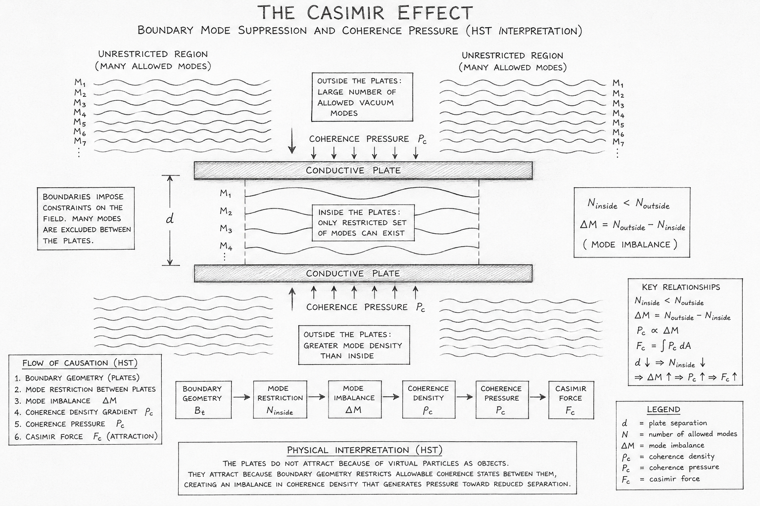
The Casimir Effect: Boundary Mode Suppression and Coherence Pressure

Overview of the Diagram

This diagram illustrates the Holographic Space-Time (HST) interpretation of the Casimir Effect. Rather than describing the attraction between conductive plates as the result of virtual particles emerging from the vacuum, the figure presents the phenomenon as a consequence of boundary-induced restrictions on allowable coherence modes.

The diagram is organised to show the complete causal pathway from physical geometry to measurable force. It begins with the conductive boundaries, progresses through mode suppression and coherence-density imbalance, and concludes with the emergence of the Casimir force.

The central scientific message is that physical attraction can arise solely from restrictions placed upon allowable field configurations.

1. Unrestricted Vacuum Regions

The upper and lower regions of the figure are labelled:

"Unrestricted Region (Many Allowed Modes)"

These areas represent space outside the conductive plates.

The multiple sinusoidal waveforms labelled:

M₁  M₂  M₃  M₄  M₅  M₆  M₇

represent the large collection of allowable field modes available in unconstrained space.

Within HST, these modes correspond to permissible coherence configurations rather than individual particles.

The abundance of modes indicates that the external region possesses a larger configuration space and therefore greater coherence freedom.

Mathematically:

Noutside​

is large.

This serves as the reference state for the entire diagram.

2. Conductive Boundary Plates

At the centre of the figure are two parallel conductive plates.

These plates are represented as rigid geometric constraints.

Their role is not to generate force.

Instead, they define allowable field behaviour.

Within HST the plates function as:

Bt​

the active boundary geometry.

The plates impose restrictions on which coherence modes can exist within the gap.

This boundary condition is the origin of every downstream effect shown in the figure.

Without boundaries there would be no Casimir phenomenon.

3. Plate Separation Distance

The distance between the plates is denoted:

d

This separation determines how many field configurations can fit between the boundaries.

As dd becomes smaller:

  • fewer standing modes survive
  • more configurations become excluded
  • the internal coherence space shrinks

The diagram therefore treats distance as a control parameter governing the degree of mode suppression.

4. Restricted Internal Region

The central cavity between the plates contains only a few standing wave structures.

These are labelled:

M₁
M₂
M₃
M₄

Unlike the external region, many possible modes are absent.

The label:

"Only Restricted Set of Modes Can Exist"

indicates that the internal coherence space is geometrically constrained.

This corresponds to:

Ninside​

where:

Ninside​<Noutside​

This inequality is the foundational condition of the Casimir Effect.

The figure visually communicates that the vacuum between the plates possesses fewer allowable configurations than the surrounding vacuum.

5. Mode Imbalance Region

On the right side of the diagram appears the relation:

\[ N_{\mathrm{inside}} < N_{\mathrm{outside}} \]

followed by:

\[ \Delta M = N_{\mathrm{outside}} - N_{\mathrm{inside}} \]

This quantity measures the magnitude of boundary-induced suppression.

Within the flow architecture:

Mode Restriction
      ↓
Delta_M

The diagram identifies this imbalance as the direct consequence of geometric constraints.

Importantly, the imbalance does not represent missing particles.

It represents missing permissible states.

6. Coherence Pressure Arrows

Large arrows labelled:

\[ P_C \]

appear above and below the conductive plates.

These arrows indicate the emergence of coherence pressure.

Within HST:

\[ P_C \propto \Delta M \]

The pressure arises because the field contains unequal configuration freedom across the boundary.

The coherence field naturally evolves toward reducing this asymmetry.

The arrows therefore represent the tendency of the geometry to relax toward a lower-tension state.

This pressure is the precursor to the observable force.

7. Coherence Density Interpretation

The diagram includes the statement:

"Outside the Plates: Greater Mode Density Than Inside"

This corresponds to the coherence-density field:

\[ \rho_C \]

The coherence density is not simply a count of modes.

It represents the distribution of informational freedom throughout the geometry.

The difference in density generates:

\[ \nabla \rho_C \]

a coherence gradient.

This gradient provides the physical basis for pressure generation.

8. Flow of Causation Block

The lower-left panel summarises the complete causal mechanism.

The sequence reads:

1. Boundary Geometry
2. Mode Restriction
3. Mode Imbalance
4. Coherence Density Gradient
5. Coherence Pressure
6. Casimir Force

This panel translates the entire diagram into a compact execution chain.

Each step follows directly from the previous one.

No force is inserted externally.

The attraction emerges naturally from the structure of the coherence field.

9. Central Flow Architecture

The centre-bottom sequence presents the formal HST execution path:

Boundary Geometry
        ↓
Mode Restriction
        ↓
Mode Imbalance
        ↓
Coherence Density
        ↓
Coherence Pressure
        ↓
Casimir Force

This section represents the operational core of the diagram.

It demonstrates that force generation is the final outcome of a chain of geometric transformations.

The sequence mirrors the corresponding Flow Algebra execution path:

B_t
→ M_inside
→ ΔM
→ ρC
→ P_C
→ F_C

10. Key Relationships Panel

The right-hand panel summarises the mathematical structure.

The equations establish:

Mode Restriction

\[ N_{\mathrm{inside}} < N_{\mathrm{outside}} \]

Mode Imbalance

\[ \Delta M = N_{\mathrm{outside}} - N_{\mathrm{inside}} \]

Pressure Generation

\[ P_C \propto \Delta M \]

Force Generation

\[ F_C = \int P_C \, dA \]

Distance Dependence

d↓⇒Ninside​↓⇒ΔM↑⇒PC​↑⇒FC​↑

These equations quantitatively connect geometry to force.

11. Physical Interpretation Panel

The large lower panel contains the conceptual interpretation of the entire figure.

Its key statement is:

The plates do not attract because virtual particles act as physical objects.

They attract because boundary geometry restricts allowable coherence states, creating an imbalance that generates pressure toward reduced separation.

This sentence encapsulates the HST reinterpretation of the Casimir Effect.

The observed force remains experimentally identical to the standard prediction.

The underlying mechanism becomes geometric rather than particle-based.

Scientific Conclusion

The diagram demonstrates that the Casimir Effect can be understood as a direct consequence of boundary-controlled coherence geometry. Conductive plates restrict the set of allowable field configurations between them, producing a mode imbalance:

\[ \Delta M = N_{\mathrm{outside}} - N_{\mathrm{inside}} \]

This imbalance generates a coherence-density gradient:

\[ \nabla \rho_C \]

which produces coherence pressure:

\[ P_C \]

The pressure integrates across the plate surfaces to create the measurable Casimir force:

\[ F_C = \int P_C \, dA \]

Within HST, the figure therefore depicts a complete causal chain in which boundary geometry creates mode restriction, mode restriction creates coherence imbalance, coherence imbalance creates pressure, and pressure manifests as physical attraction.

The Casimir Effect becomes a natural example of how measurable forces emerge from the organisation of permissible boundary states rather than from the exchange of physical vacuum particles.

Flow Mapping Table

Diagram Element Flow Symbol Scientific Meaning
Two conductive plates B_t Active boundary geometry constraining the field
Plate separation d Distance controlling allowed internal modes
Outer wave modes M_outside Unrestricted vacuum/coherence modes outside plates
Inner wave modes M_inside Restricted modes surviving between plates
Missing inner modes Mode_Suppression Boundary exclusion of incompatible configurations
Mode count inequality N_inside < N_outside Internal state-space reduction
Mode imbalance box Delta_M Suppression magnitude: N_outside − N_inside
Coherence density label rho_C Spatial distribution of allowed coherence freedom
Density gradient Gradient(rho_C) Directional imbalance in coherence structure
Pressure arrows P_C Coherence pressure generated by mode imbalance
Surface integration Integrate(P_C, A) Pressure accumulated across plate area
Casimir force F_C Observable attractive force between plates
Inward motion tendency d ↓ Relaxation toward reduced separation
Causal flow strip Execution_Path Full HST sequence from boundary to force
Key relationship panel Equations Mathematical constraints governing execution
Physical interpretation panel HST_Reinterpretation Conceptual replacement of virtual-particle explanation

Compressed Mapping Chain
Diagram:
Plates → Restricted Inner Waves → Mode Imbalance → Pressure Arrows → Attraction

Flow:
B_t → M_inside → Delta_M → P_C → F_C

Equation:
N_inside < N_outside → ΔM = N_outside - N_inside → P_C ∝ ΔM → F_C = ∫P_C dA

Execution Meaning
B_t
→ Apply_Boundary_Restrictions(M, d)
→ M_inside
→ Delta_M
→ rho_C
→ Gradient(rho_C)
→ P_C
→ F_C
→ CASIMIR_ATTRACTION

Execution Guarantee Statement

Formal Execution Guarantee

The CasimirEffect_BoundaryModeSuppression flow is guaranteed to execute successfully if and only if a valid boundary geometry exists that restricts the allowable internal coherence modes relative to the surrounding field configuration.

Execution proceeds deterministically through the sequence:

B_t
→ M_inside
→ Delta_M
→ rho_C
→ Gradient(rho_C)
→ P_C
→ F_C
→ CASIMIR_ATTRACTION

provided all stability constraints remain satisfied throughout the computation.

Boundary Existence Guarantee

Execution requires the existence of conductive boundaries:

\[ B_t \neq \emptyset \]

and a non-zero separation:

\[ d > 0 \]

Without boundary geometry there can be no mode restriction.

Therefore:

B_t = ∅
⇒ Execution = FAIL

Mode Restriction Guarantee

The flow requires that the boundary geometry suppresses allowable internal modes.

The fundamental execution condition is:

\[ N_{\mathrm{inside}} < N_{\mathrm{outside}} \]

If the internal and external mode spaces become identical:

Ninside​=Noutside​

then:

\[ \Delta M = 0 \]

and no Casimir effect can emerge.

Therefore:

Ninside ≥ Noutside
⇒ Execution = FAIL

Mode Imbalance Guarantee

The flow guarantees pressure generation whenever a valid mode imbalance exists.

The imbalance is defined as:

\[ \Delta M = N_{\mathrm{outside}} - N_{\mathrm{inside}} \]

and must satisfy:

\[ \Delta M > 0 \]

This ensures that a coherence asymmetry exists between the internal and external regions.

Coherence Density Guarantee

The suppressed mode space must produce a stable coherence-density field:

\[ \rho_C \geq C_{\mathrm{min}} \]

where:

CminC_{min} is the minimum coherence threshold

This condition guarantees that the field remains physically interpretable and structurally stable.

If:

\[ \rho_C < C_{\mathrm{min}} \]

then:

Execution = FAIL

Gradient Formation Guarantee

A valid coherence gradient must emerge from the mode imbalance:

\[ \nabla \rho_C \neq 0 \]

This gradient provides the physical mechanism through which pressure develops.

No gradient implies:

\[ P_C = 0 \]

and therefore:

\[ F_C = 0 \]

Thus:

Gradient(rho_C) = 0
⇒ No Casimir Effect

Pressure Generation Guarantee

Given:

\[ \Delta M > 0 \]

the flow guarantees formation of coherence pressure:

\[ P_C \propto \Delta M \]

This pressure is a deterministic consequence of mode suppression.

No additional force source is required.

Force Emergence Guarantee

Provided pressure exists over a finite plate area:

\[ A > 0 \]

the force calculation:

\[ F_C = \int P_C \, dA \]

guarantees a non-zero attractive interaction.

Thus:

P_C > 0
∧ A > 0
⇒ F_C > 0

Distance Dependence Guarantee

The flow guarantees the experimentally observed scaling behaviour.

As plate separation decreases:

\[ d \downarrow \]

the allowable internal mode count decreases:

\[ N_{\mathrm{inside}} \downarrow \]

which yields:

\[ \Delta M \uparrow \]

therefore:

\[ P_C \uparrow \]

and:

\[ F_C \uparrow \]

Thus the attraction strengthens automatically without introducing additional mechanisms.

Conservation Guarantee

The flow does not create or destroy coherence.

Instead it redistributes allowable configurations through geometric constraints.

Therefore:

Total Coherence=Conserved

while:

Local Mode Density=Redistributed

This ensures consistency with HST conservation principles.

Failure Conditions

Execution terminates if any of the following occur:

B_t = ∅

d ≤ 0

Ninside ≥ Noutside

Delta_M ≤ 0

rho_C < Cmin

Gradient(rho_C) = 0

P_C = 0

F_C = 0

These conditions remove the geometric asymmetry necessary for Casimir force generation.

Guaranteed Execution Path

B_t
→ Boundary Restriction
→ M_inside
→ Ninside < Noutside
→ Delta_M
→ rho_C
→ Gradient(rho_C)
→ P_C
→ F_C
→ CASIMIR_ATTRACTION
Telephone:
01377 236594

Formal HST Guarantee Statement

\[ B_t \neq \emptyset \]

\[ d > 0 \]

\[ N_{\mathrm{inside}} < N_{\mathrm{outside}} \]

\[ \Delta M > 0 \]

\[ \rho_C \geq C_{\mathrm{min}} \]

\[ \nabla \rho_C \neq 0 \]

\[ P_C \propto \Delta M \]

\[ F_C = \int P_C \, dA > 0 \]

∴

Execution(Pt​)=CASIMIR_ATTRACTION


Execution Result

Under the stated constraints, the flow is guaranteed to produce a stable Casimir attraction through boundary-induced mode suppression, coherence-density imbalance, pressure generation, and force emergence.

Within HST, the effect arises deterministically from boundary geometry and coherence minimisation, requiring no virtual-particle mechanism to achieve execution.

Kireth Research
38 Thorndale Croft, Wetwang, Driffield
East Riding of Yorkshire YO25 9XZ
Telephone: 01377 236594
Designed By