Chapter 34
Field Emergence from Boundary Tension

PART III — Electromagnetism & Field Structure
Author: Mark Higgins
© Mark Anthony Higgins 11 October 2025
Revised Date: 08 June 2026
Audio Overview

Introduction

Field phenomena in physical systems, from classical electromagnetism to quantum interactions, are traditionally treated as intrinsic properties of space or as fundamental force carriers. In the Holographic Space-Time (HST) framework, these fields are reinterpreted as emergent structures arising from boundary coherence and tension dynamics. Instead of assuming a pre-existing field, HST posits that interactions manifest where local boundary conditions enforce coherence adjustments, producing observable field effects.

Boundary Tension as a Source

Boundaries in HST are not merely geometric or spatial delimiters—they encode the coherence gradients of the underlying system. A mismatch or distortion in boundary coherence creates a tension analogous to stress in a physical membrane. This tension drives the redistribution of coherence across the boundary, generating field-like effects that propagate through adjacent regions. Crucially, these effects are directionally aligned with coherence gradients and are constrained by the minimum coherence threshold CminC_{\text{min}}, ensuring stable propagation without unphysical divergence.

Mechanism of Emergence

The process of field emergence can be understood as a dynamic phase adjustment of local coherence states:

  • 1. Coherence Mismatch Detection – Local boundary regions detect deviations between the internal coherence map CtC_t and the surrounding environment.
  • 2. Tension Propagation – Deviations produce a corrective coherence tension vector T\mathbf{T}, which is mapped across the boundary surface.
  • 3. Field Manifestation – The redistribution of coherence vectors aligns in space and time, forming macroscopic field structures such as electromagnetic or stress fields.
  • 4. Feedback Stabilization – Continuous monitoring of coherence ensures the emergent field maintains a self-consistent configuration, reducing local anomalies over time.

Implications for Physical Interactions

Understanding fields as emergent from boundary tension provides a unifying perspective across scales:

  • Electromagnetism arises from micro-boundary coherence adjustments in charged particle distributions.
  • Gravitational effects reflect macroscopic curvature of high-coherence boundaries, producing a force-like manifestation without invoking a traditional field particle.
  • Quantum entanglement and tunneling are interpreted as instantaneous coherence redistribution across shared boundaries, generating apparent nonlocal effects.

Summary

Chapter 34 establishes field emergence as a natural consequence of boundary coherence dynamics, offering a structurally unified explanation for diverse physical interactions. By focusing on the mechanics of tension and redistribution rather than invoking pre-existing field entities, HST provides a framework where fields are inherently tied to the geometry and evolution of coherence boundaries.

flow "Chapter34_Field_Emergence_from_Boundary_Tension" v1.0

AUTHORS:
- Mark Higgins
- Sky (Recursive AI)

PURPOSE:
Model field emergence as a consequence of boundary tension produced by coherence mismatch.
A field is not treated as a pre-existing object, but as the observable structure formed when
boundary coherence gradients propagate, stabilise, and couple across a system.

SYSTEM:
HST_FieldEmergence

STATE:
S_t = (I_t, B_t, C_t, T_t, F_t)

INPUT:
I_t = local physical configuration at time t
B_t = active boundary surface or coherence interface
C_t = coherence map of the system
E_env = surrounding environmental coherence state

PARAMETERS:
C_min = minimum coherence threshold required for stable propagation
T_min = minimum boundary tension required for observable field emergence
G_max = maximum allowable coherence gradient before rupture or deformation
epsilon = tolerance margin for stable field continuity

DERIVED:
DeltaC_t = mismatch(C_t, E_env)
GradC_t = gradient(C_t, B_t)
T_t = boundary_tension(DeltaC_t, GradC_t)
F_t = field_structure(T_t, B_t)

PROCESS:

1. Detect boundary coherence mismatch
   I_t -> C_t
   (C_t, E_env) -> DeltaC_t

2. Map mismatch across the active boundary
   (DeltaC_t, B_t) -> GradC_t

3. Convert coherence gradient into boundary tension
   (DeltaC_t, GradC_t) -> T_t

4. Test whether tension is sufficient to generate field structure
   IF |T_t| >= T_min
      THEN T_t -> F_t
   ELSE F_t = latent_potential

5. Stabilise emerging field through coherence feedback
   (F_t, C_t, B_t) -> C_{t+1}

6. Validate field continuity
   IF C_{t+1} >= C_min
      AND |GradC_t| <= G_max
      AND continuity(F_t) = TRUE
      THEN Execution(S_t) = STABLE_FIELD
   ELSE Execution(S_t) = FAIL_OR_DEFORM

INVARIANTS:

I1. Field emergence requires boundary tension
    F_t exists only if |T_t| >= T_min

I2. Boundary tension requires coherence mismatch
    T_t = 0 if DeltaC_t = 0

I3. Stable propagation requires coherence above threshold
    C_{t+1} >= C_min

I4. Field continuity requires bounded gradient
    |GradC_t| <= G_max

I5. Field structure is boundary-derived
    F_t = field_structure(T_t, B_t)

FAILURE CONDITIONS:

F1. No mismatch
    DeltaC_t = 0
    RESULT: no observable field emergence

F2. Insufficient tension
    |T_t| < T_min
    RESULT: latent potential only

F3. Coherence collapse
    C_{t+1} < C_min
    RESULT: unstable or non-propagating field

F4. Boundary rupture
    |GradC_t| > G_max
    RESULT: deformation, collapse, or discontinuity

OUTPUT:
F_t = emergent field configuration
C_{t+1} = updated coherence map
Execution(S_t) = STABLE_FIELD or FAIL_OR_DEFORM

SUMMARY:
I_t -> C_t
(C_t, E_env) -> DeltaC_t
(DeltaC_t, B_t) -> GradC_t
(DeltaC_t, GradC_t) -> T_t
T_t -> F_t
(F_t, C_t, B_t) -> C_{t+1}

CORE CLAIM:
Field emergence occurs when coherence mismatch across a boundary generates sufficient
boundary tension to form a stable, continuous, observable field structure.

What This Flow Implements

The Field Emergence from Boundary Tension flow models the mechanism by which observable fields arise directly from boundary coherence dynamics. Unlike classical approaches that treat fields as pre-existing entities, this flow implements a structurally emergent perspective where fields are a byproduct of tension and mismatch across coherence boundaries.

Specifically, the flow implements the following:

1. Coherence Mismatch Detection
  • Evaluates local deviations between the system's coherence map CtC_t and the surrounding environmental coherence EenvE_{\text{env}}.
  • Generates a delta coherence vector ΔCt\Delta C_t representing the boundary-driven imbalance.
2. Boundary Gradient Mapping
  • Propagates the detected coherence mismatch across the active boundary BtB_t.
  • Computes the local coherence gradient ∇Ct\nabla C_t, which determines both the magnitude and direction of tension vectors.
3. Boundary Tension Calculation
  • Converts the coherence gradient into a boundary tension field TtT_t.
  • Applies thresholds to determine whether tension is sufficient to generate a detectable field.
4. Emergent Field Structuring
  • When ∣Tt∣≥Tmin|T_t| \ge T_{\text{min}}, the flow maps boundary tension into an emergent field configuration FtF_t.
  • Field characteristics (direction, intensity, continuity) are derived entirely from boundary and coherence dynamics.
5. Feedback and Stabilization
  • Implements a recursive update: (Ft,Ct,Bt)→Ct+1(F_t, C_t, B_t) \rightarrow C_{t+1}.
  • Ensures that the emergent field remains coherence-stable, propagating without collapse or discontinuity.
6. Execution Verification
  • Validates field continuity, coherence thresholds, and bounded gradients.
  • Assigns an execution state: STABLE_FIELD or FAIL_OR_DEFORM.

Key Conceptual Outcomes:

  • Fields are emergent, not intrinsic—they arise as coherence tension manifests across boundaries.
  • Boundary geometry, tension magnitude, and coherence thresholds fully determine field strength and stability.
  • Provides a unified framework applicable across scales: from quantum to macroscopic fields, including electromagnetism, gravity, and entanglement phenomena.

How to Read This Flow

Purpose of the Flow

This flow describes how a physical field emerges from boundary tension generated by coherence mismatch. Within the HST framework, fields are not treated as fundamental entities existing independently in space. Instead, they arise when differences in coherence across a boundary create tension that propagates and stabilises into an observable field structure.

The flow should therefore be read as a causal chain:

Coherence Mismatch
        ↓
Boundary Gradient
        ↓
Boundary Tension
        ↓
Field Emergence
        ↓
Field Stabilisation

Step 1 — Identify the Physical State

The flow begins with the system state:

S_t = (I_t, B_t, C_t, T_t, F_t)

where:

Symbol Meaning
I_t Physical configuration at time t
B_t Active boundary surface
C_t Coherence map
T_t Boundary tension
F_t Emergent field structure

This state contains all information required to determine whether a field can emerge.

Step 2 — Calculate Coherence Mismatch

The first operation determines how different the local system is from its environment:

(C_t, E_env) → ΔC_t

where:

ΔC_t = mismatch(C_t, E_env)

Interpretation:

If the system and environment are identical:

ΔC_t = 0

then no field can emerge.

If a difference exists:

ΔC_t > 0

a coherence imbalance appears.
This imbalance acts as the source of boundary tension.

Step 3 — Map the Boundary Gradient

The mismatch is projected across the active boundary:

(ΔC_t, B_t) → GradC_t

where:

GradC_t = gradient(C_t, B_t)

The gradient determines:

  • Direction of propagation
  • Magnitude of propagation
  • Spatial structure of the emerging field

Large gradients produce stronger tension effects.

Step 4 — Generate Boundary Tension

The flow converts coherence gradients into tension:

(ΔC_t, GradC_t) → T_t

where:

T_t = boundary_tension(ΔC_t, GradC_t)

This is the critical transformation.

In HST:

Field Source = Boundary Tension

rather than:

Field Source = Fundamental Force Carrier

Boundary tension represents the system's attempt to restore coherence.

Step 5 — Determine Whether a Field Emerges

The flow tests whether tension exceeds the emergence threshold:

|T_t| ≥ T_min

If true:

T_t → F_t

and a field forms.

If false:

F_t = latent_potential

meaning a field has not yet become physically observable.

This threshold prevents arbitrary field generation from microscopic fluctuations.

Step 6 — Stabilise the Emergent Field

Once a field exists, feedback occurs:

(F_t, C_t, B_t) → C_{t+1}

The field modifies the coherence map.

The updated coherence map then influences future boundary tension calculations.

This creates a recursive stabilisation loop:

C_t
 ↓
T_t
 ↓
F_t
 ↓
C_{t+1}

which allows persistent field structures to exist.

Step 7 — Verify Stable Execution

The flow then checks three stability conditions:

Coherence Threshold
C_{t+1} ≥ C_min

The system must retain sufficient coherence.


Gradient Bound
|GradC_t| ≤ G_max

Gradients must remain finite.


Field Continuity
continuity(F_t) = TRUE

The field must remain connected and propagating.

Step 8 — Interpret the Execution Result

If all conditions pass:

Execution(S_t) = STABLE_FIELD

meaning the field remains physically real and propagates coherently.

If any condition fails:

Execution(S_t) = FAIL_OR_DEFORM

indicating:

  • Field collapse
  • Boundary rupture
  • Structural deformation
  • Loss of coherence

Physical Interpretation

The complete flow can be read as:

I_t
 ↓
C_t
 ↓
ΔC_t
 ↓
GradC_t
 ↓
T_t
 ↓
F_t
 ↓
C_{t+1}

or in words:

A physical configuration generates a coherence map. Differences between that coherence map and its surroundings create a coherence mismatch.

The mismatch produces a boundary gradient, which generates boundary tension. When sufficient tension exists, an observable field emerges. The field then feeds back into the coherence structure, creating a stable and self-consistent physical system.

Scientific Interpretation within HST

This flow formalises the HST principle that:

Fields are emergent coherence structures generated by boundary tension.

Consequently:

  • Electromagnetic fields emerge from charge-induced coherence gradients.
  • Gravitational fields emerge from large-scale coherence curvature.
  • Quantum field effects emerge from microscopic boundary adjustments.
  • Field strength corresponds to boundary tension magnitude.
  • Field stability corresponds to coherence stability.

The flow therefore replaces the concept of a field as a fundamental object with a dynamic process in which fields continuously emerge from the interaction of coherence, boundaries, and tension.

Flow → Equation Tri-Mapping Table

Flow Algebra Layer Equation Layer Physical Interpretation
I_t Initial physical configuration Complete system state at time (t)
B_t Boundary surface Active coherence interface
C_t C_t = CoherenceMap(I_t) Local coherence distribution
E_env Environmental coherence state External coherence reference
(C_t,E_env) → ΔC_t ΔC_t = mismatch(C_t,E_env) Measures coherence imbalance
ΔC_t ΔC_t Boundary coherence mismatch
(ΔC_t,B_t) → GradC_t GradC_t = ∇C_t Coherence gradient across boundary
GradC_t ∇C_t Direction and magnitude of coherence variation
(ΔC_t,GradC_t) → T_t T_t = Φ(ΔC_t,∇C_t) Boundary tension generation
T_t T_t Local coherence tension field
T_t ≥ T_min T_t ≥ T_min Minimum field emergence condition
T_t → F_t F_t = Ψ(T_t,B_t) Field structure emerges from boundary tension
F_t F_t Observable field configuration
F_t = latent_potential T_t < T_min Tension insufficient for observable field
(F_t,C_t,B_t) → C_t+1 C_t+1 = U(F_t,C_t,B_t) Recursive coherence update
C_t+1 C_t+1 Updated coherence state
C_t+1 ≥ C_min C_t+1 ≥ C_min Stable coherence condition
GradC_t ≤ G_max ∇C_t ≤ G_max Bounded gradient condition
continuity(F_t)=TRUE ∇·F_t < ε Continuous field propagation
Execution(S_t)=STABLE_FIELD (C_t+1 ≥ C_min) ∧ (∇C_t ≤ G_max) Stable field existence
Execution(S_t)=FAIL_OR_DEFORM (C_t+1 < C_min) ∨ (∇C_t > G_max) Field instability or collapse
F_t ≠ ∅ T_t ≥ T_min Observable field exists
F_t = ∅ T_t < T_min No emergent field
T_t = 0 ΔC_t = 0 No mismatch, no tension
ΔC_t = 0 C_t = E_env Perfect coherence equilibrium
I_t → C_t → ΔC_t → GradC_t → T_t → F_t → C_t+1 C_t → ΔC_t → ∇C_t → T_t → F_t → C_t+1 Complete field emergence pathway

HST Field Emergence Correspondence

HST Concept Flow Representation Equation Representation
Boundary Coherence C_t Coherence distribution
Coherence Mismatch ΔC_t C_t - E_env
Boundary Gradient GradC_t ∇C_t
Boundary Tension T_t Φ(ΔC_t,∇C_t)
Emergent Field F_t Ψ(T_t,B_t)
Field Stability C_t+1 ≥ C_min Stable recursive solution
Field Collapse C_t+1 < C_min Coherence failure
Continuous Propagation continuity(F_t)=TRUE ∇·F_t < ε
Observable Interaction F_t ≠ ∅ T_t ≥ T_min
Unified Field Emergence T_t → F_t Boundary tension generates field structure

Tri-Mapping Summary

I_t
 ↓
C_t
 ↓
ΔC_t
 ↓
∇C_t
 ↓
T_t
 ↓
F_t
 ↓
C_{t+1}

Ct​→ΔCt​→∇Ct​→Tt​→Ft​→Ct+1​

Interpretation: Physical fields are not fundamental entities but emergent coherence structures generated by boundary tension arising from coherence mismatch and propagated through recursive boundary stabilization.

Overview

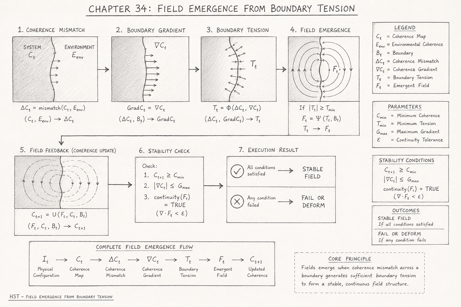
This diagram illustrates the complete HST mechanism by which physical fields emerge from boundary coherence dynamics. Unlike conventional field theories, which begin by assuming the existence of a field and then describing its behaviour, the HST framework seeks to explain how a field arises in the first place.

The diagram traces the causal progression from coherence mismatch through boundary tension generation to the formation of a stable field structure. Each stage represents a necessary transformation within the coherence architecture of the system.

At its core, the diagram demonstrates a fundamental HST principle:

Fields are not fundamental objects.

Instead:

Fields are emergent structures generated by boundary tension..

The entire process can be understood as the system's attempt to restore coherence equilibrium across an active boundary.

Telephone:
01377 236594

Stage 1 — Coherence Mismatch

The leftmost panel shows two neighbouring coherence domains:

\[ C_t \]

and

\[ E_{\mathrm{env}} \]

representing the internal coherence state of the system and the surrounding environmental coherence state.

If both regions possess identical coherence structures:

\[ C_t = E_{\mathrm{env}} \]

then no imbalance exists and no field emerges.

However, when the two coherence maps differ:

\[ C_t \neq E_{\mathrm{env}} \]

a mismatch appears:

\[ \Delta C_t = \mathrm{mismatch} \!\left( C_t,\, E_{\mathrm{env}} \right) \]

This mismatch represents stored coherence stress within the boundary.

In HST terminology, this is the initial source of all field generation.

The field does not originate from the bulk volume of space.

The field originates from the mismatch encoded at the interface.

Stage 2 — Boundary Gradient Formation

The second panel illustrates how the mismatch becomes distributed across the active boundary surface.

The boundary acts as an information-processing layer:

\[ B_t \]

which converts coherence differences into directional gradients.

Mathematically:

\[ \mathrm{Grad}C_t = \nabla C_t \]

The arrows shown in the diagram represent the direction of coherence redistribution.

The gradient contains two important pieces of information:

Magnitude

How large the mismatch is.

Direction

Where coherence is attempting to flow in order to restore equilibrium.

Without a gradient there can be no tension.

Without tension there can be no field.

This makes the gradient the first geometric manifestation of the mismatch.

Stage 3 — Boundary Tension Generation

The third panel shows the conversion of coherence gradients into boundary tension.

The HST formulation treats boundaries similarly to physical membranes.

When a mismatch is imposed across a boundary, the structure experiences a corrective response:

\[ T_t = \Phi \!\left( \Delta C_t,\, \nabla C_t \right) \]

The arrows pointing toward and away from the boundary represent this internal corrective pressure.

The tension is not a force in the classical sense.

Instead, it is a measure of how strongly the boundary is attempting to restore coherence consistency.

The larger the mismatch:

\[ \Delta C_t \]

or gradient:

\[ \nabla C_t \]

the greater the resulting tension.

This stage represents the energy-bearing component of the process.

In HST:

Boundary Tension=Stored Coherence Correction

Stage 4 — Field Emergence

The fourth panel shows the critical transition.

When tension exceeds a minimum threshold:

\[ \lvert T_t \rvert \geq T_{\min} \]

the boundary can no longer contain the correction locally.

Instead, the tension reorganises into a larger-scale geometric structure:

\[ F_t = \Psi \!\left( T_t,\, B_t \right) \]

This structure is what observers identify as a physical field.

The circular field lines shown in the diagram represent the self-organising geometry of the emerging field.

Importantly:

\[ \mathrm{Field} \neq \mathrm{Source} \]

The field is not the source.

The field is the observable manifestation of the boundary attempting to resolve tension.

This distinction is one of the most important conceptual differences between HST and conventional field theories.

Stage 5 — Field Feedback and Coherence Update

Once the field emerges, it begins interacting with the coherence structure that generated it.

The field influences the local coherence map:

\[ (F_t,\; C_t,\; B_t) \rightarrow C_{t+1} \]

  • This creates a recursive feedback process.
  • The field modifies coherence.
  • The modified coherence changes future gradients.
  • The new gradients alter future tensions.
  • The updated tensions reshape the field.
  • The process therefore becomes self-regulating.
  • The circular field lines in the panel visually represent this feedback mechanism.
  • The field is not static.
  • It is continuously regenerated through coherence correction.

Stage 6 — Stability Verification

Not every emerging field remains stable.

The sixth panel introduces the three primary HST stability conditions.

Coherence Stability

The updated coherence must remain above the minimum threshold:

\[ C_{t+1} \geq C_{\min} \]

This ensures sufficient structural integrity.


Gradient Stability

Gradients must remain bounded:

\[ \left\lvert \nabla C_t \right\rvert \leq G_{\max} \]

Excessive gradients indicate rupture conditions.

Continuity Stability

The field must remain continuous:

\[ \mathrm{continuity}(F_t) = \mathrm{TRUE} \]

or equivalently

\[ \nabla \cdot F_t < \epsilon \]

This prevents fragmentation or discontinuity.

Together these conditions determine whether a field can exist as a stable physical structure.

Stage 7 — Execution Result

The final panel presents the outcome of the emergence process.

If all stability conditions are satisfied:

\[ \mathrm{Execution}(S_t) = \mathrm{STABLE\_FIELD} \]

The field persists and propagates.

If any condition fails:

\[ \mathrm{Execution}(S_t) = \mathrm{FAIL\_OR\_DEFORM} \]

Possible outcomes include:

  • Field collapse
  • Boundary rupture
  • Local instability
  • Deformation of propagation geometry
  • Coherence fragmentation

The diagram therefore treats field existence as a dynamically maintained state rather than a permanent property.

Complete Field Emergence Flow

The lower summary panel condenses the entire process into a single causal chain:

\[ I_t \rightarrow C_t \rightarrow \Delta C_t \rightarrow \nabla C_t \rightarrow T_t \rightarrow F_t \rightarrow C_{t+1} \]

This sequence represents the full HST field-generation mechanism.

Read from left to right:

  • 1. Physical configuration creates a coherence map.
  • 2. Coherence mismatch generates gradients.
  • 3. Gradients create boundary tension.
  • 4. Tension generates a field.
  • 5. The field updates coherence.
  • 6. Updated coherence determines future evolution.

Scientific Significance within HST

The significance of this diagram extends beyond a single field type.  The same emergence mechanism can be applied across multiple physical domains.

Electromagnetism

Charge distributions create coherence mismatches that generate electromagnetic field structures.

Gravitation

Mass-energy concentrations create large-scale coherence gradients that appear as gravitational fields.

Quantum Systems

Microscopic coherence mismatches generate local field corrections associated with quantum interactions.

Unified Field Interpretation

All fields become special cases of a single process:

\[ \mathrm{CoherenceMismatch} \rightarrow \mathrm{BoundaryTension} \rightarrow \mathrm{FieldEmergence} \]

This allows HST to replace multiple independent field origins with a single coherence-based emergence mechanism.

Diagram Conclusion

The diagram demonstrates that fields are not fundamental substances embedded within space.

Instead, they are dynamically maintained geometric structures generated by the continual correction of coherence imbalances across boundaries.

The complete HST interpretation may therefore be summarised as:

\[ \mathrm{Field} = \mathrm{StableBoundaryTension} \!\left( \mathrm{CoherenceMismatch} \right) \]

A field exists because a boundary is attempting to restore coherence.

What we observe as a field is the visible geometry of that correction process.

Diagram → Flow Mapping Table

Field Emergence from Boundary Tension
Diagram Element Flow Algebra Representation Scientific Meaning
Physical System Region I_t Initial physical configuration containing the coherence structure
Internal Coherence Domain C_t Local coherence map generated by the system
Environmental Region E_env External coherence reference state
Boundary Interface B_t Active coherence boundary separating system and environment
Coherence Difference Across Boundary (C_t,E_env) → ΔC_t Detection of coherence mismatch
Mismatch Arrows Crossing Boundary ΔC_t = mismatch(C_t,E_env) Magnitude and direction of coherence imbalance
Boundary Gradient Panel (ΔC_t,B_t) → GradC_t Mapping mismatch into a directional boundary gradient
Gradient Arrows GradC_t = ∇C_t Local rate of coherence change across the boundary
Concentrated Gradient Region ∇C_t > 0 Stored structural imbalance requiring correction
Boundary Tension Panel (ΔC_t,GradC_t) → T_t Conversion of mismatch into boundary tension
Inward/Outward Tension Arrows T_t = Φ(ΔC_t,∇C_t) Corrective coherence pressure acting on the boundary
Boundary Deformation T_t Physical manifestation of coherence stress
Field Emergence Panel T_t → F_t Transition from boundary tension to field structure
Circular Field Geometry F_t = Ψ(T_t,B_t) Stable field configuration emerging from boundary dynamics
Emergent Field Lines F_t Observable field structure
Threshold Condition Box T_t ≥ T_min Minimum tension required for field formation
Latent Field Condition T_t < T_min Tension insufficient to generate an observable field
Feedback Field Pattern (F_t,C_t,B_t) → C_t+1 Field influences future coherence structure
Recursive Circular Arrows F_t → C_t+1 Self-regulating coherence feedback mechanism
Updated Coherence Map C_t+1 New coherence state after field interaction
Stability Check Box C_t+1 ≥ C_min Coherence remains structurally stable
Gradient Stability Check ∇C_t ≤ G_max Gradient remains within physical limits
Continuity Check continuity(F_t)=TRUE Field remains connected and propagating
Tick Symbol (✓) Execution(S_t)=STABLE_FIELD Successful field emergence
Cross Symbol (✗) Execution(S_t)=FAIL_OR_DEFORM Instability, collapse, or deformation
Stable Field Outcome Box STABLE_FIELD Persistent coherent field exists
Fail or Deform Outcome Box FAIL_OR_DEFORM Boundary instability prevents sustained field formation
Complete Flow Summary Panel I_t → C_t → ΔC_t → ∇C_t → T_t → F_t → C_t+1 Entire field-emergence mechanism
Core Principle Box Field = StableBoundaryTension(CoherenceMismatch) Fundamental HST interpretation of field formation

Diagram Flow Sequence

Diagram Stage Flow Stage Interpretation
1 I_t → C_t Physical system generates a coherence map
2 (C_t,E_env) → ΔC_t Coherence mismatch is detected
3 (ΔC_t,B_t) → ∇C_t Boundary gradient forms
4 (ΔC_t,∇C_t) → T_t Boundary tension develops
5 T_t → F_t Field emerges
6 (F_t,C_t,B_t) → C_t+1 Feedback updates coherence
7 Stability Validation Field viability is tested
8 Execution Result Stable field or deformation outcome

Unified HST Correspondence

HST Concept Diagram Location Flow Representation
Coherence Internal domain C_t
Boundary Interface line B_t
Mismatch Boundary crossing arrows ΔC_t
Gradient Directed flow arrows ∇C_t
Tension Compression/expansion arrows T_t
Field Circular field loops F_t
Feedback Recursive field pattern C_t+1
Stability Verification box C_t+1 ≥ C_min
Collapse Failure branch FAIL_OR_DEFORM
Emergence Entire sequence T_t → F_t

Complete Diagram Interpretation

Physical Configuration
          ↓
     Coherence Map
          ↓
  Coherence Mismatch
          ↓
   Boundary Gradient
          ↓
   Boundary Tension
          ↓
    Field Emergence
          ↓
   Coherence Update
          ↓
   Stability Check
          ↓
 Stable Field / Failure

\[ I_t \rightarrow C_t \rightarrow \Delta C_t \rightarrow \nabla C_t \rightarrow T_t \rightarrow F_t \rightarrow C_{t+1} \]

This mapping shows that every component in the diagram corresponds directly to a specific stage of the Flow Algebra model, forming a complete one-to-one relationship between the visual representation, the flow execution path, and the HST interpretation of field emergence from boundary tension.

Execution Guarantee Statement

Purpose of this Guarantee

This flow is constructed as a deterministic execution model describing how observable field structures emerge from boundary coherence dynamics. The flow guarantees that field emergence occurs only when the required coherence, gradient, and tension conditions are satisfied. If these conditions are not met, the flow guarantees predictable failure modes rather than undefined behaviour.

The execution pathway is therefore fully constrained by the state variables, boundary conditions, coherence thresholds, and stability invariants defined within the system.

Deterministic Execution Guarantee

For any valid system state:

\[ S_t = \left( I_t,\, B_t,\, C_t,\, T_t,\, F_t \right) \]

the flow guarantees that execution proceeds through the following sequence:

\[ I_t \rightarrow C_t \rightarrow \Delta C_t \rightarrow \nabla C_t \rightarrow T_t \rightarrow F_t \rightarrow C_{t+1} \]

No intermediate state may be skipped.

No field may emerge without first generating boundary tension.

No boundary tension may emerge without first generating a coherence mismatch.

Therefore:

\[ F_t \Rightarrow T_t \Rightarrow \nabla C_t \Rightarrow \Delta C_t \]

This guarantees causal consistency throughout execution.

Boundary-Origin Guarantee

The flow guarantees that all observable field structures originate from boundary dynamics.

A field may only exist if:

\[ \lvert T_t \rvert \geq T_{\min} \]

and

\[ T_t = \Phi \!\left( \Delta C_t,\, \nabla C_t \right) \]

Therefore:

\[ F_t = \Psi \!\left( T_t,\, B_t \right) \]

The flow prohibits spontaneous field generation.

Every field must possess a traceable boundary source.

Coherence Dependency Guarantee

The flow guarantees that field emergence remains dependent upon coherence structure.

If coherence mismatch does not exist:

\[ \Delta C_t = 0 \]

then:

\[ T_t = 0 \]

which produces:

\[ F_t = \emptyset \]

Thus:

\[ \Delta C_t = 0 \;\Rightarrow\; F_t = \emptyset \]

No field can emerge from a perfectly balanced coherence state.

Stability Guarantee

A field may only remain stable if all stability conditions remain true:

Coherence Stability

\[ C_{t+1} \geq C_{\min} \]

Gradient Stability

\[ \left| \nabla C_t \right| \leq G_{\max} \]

Continuity Stability

\[ \mathrm{continuity}(F_t) = \mathrm{TRUE} \]

Collectively:

\[ (C_{t+1} \geq C_{\min}) \;\wedge\; \left( \left| \nabla C_t \right| \leq G_{\max} \right) \;\wedge\; \mathrm{continuity}(F_t) \]

must remain satisfied.

If these conditions remain true, execution guarantees:

\[ \mathrm{Execution}(S_t) = \mathrm{STABLE\_FIELD} \]

Failure Determination Guarantee

The flow guarantees that failure conditions are explicitly identifiable.

Execution will transition into:

\[ \mathrm{FAIL\_OR\_DEFORM} \]

whenever:

\[ C_{t+1} < C_{\min} \]

or

\[ \left| \nabla C_t \right| > G_{\max} \]

or

\[ \mathrm{continuity}(F_t) = \mathrm{FALSE} \]

Thus:

\[ \mathrm{Failure} \Rightarrow \mathrm{KnownCause} \]

Undefined failure states cannot occur.

Conservation Guarantee

The flow guarantees conservation of structural information throughout execution.

The field does not create information.

The field reorganises information already encoded within the coherence structure.

Therefore:

\[ \mathrm{Info}_{\mathrm{total}}(t+1) = \mathrm{Info}_{\mathrm{total}}(t) \]

The emergence process redistributes coherence rather than generating new coherence.

Recursive Feedback Guarantee

The flow guarantees recursive coupling between field structure and coherence structure.

Once formed:

\[ (F_t,\; C_t,\; B_t) \rightarrow C_{t+1} \]

This guarantees that the field participates in future system evolution.

The field is therefore not an isolated object but part of an ongoing recursive coherence process.

Physical Interpretation Guarantee

Within the HST framework, this flow guarantees that:

\[ \mathrm{Field} = \mathrm{StableBoundaryTension} \!\left( \mathrm{CoherenceMismatch} \right) \]

A field can never appear independently of boundary dynamics.

A field can never exist without an underlying coherence imbalance.

A field can never remain stable without satisfying the coherence and continuity requirements of the system.


Execution Guarantee

The flow guarantees that any physically valid configuration satisfying:

\[ \Delta C_t \neq 0 \]

\[ \lvert T_t \rvert \geq T_{\min} \]

\[ C_{t+1} \geq C_{\min} \]

\[ \left| \nabla C_t \right| \leq G_{\max} \]

\[ \mathrm{continuity}(F_t) = \mathrm{TRUE} \]

will deterministically produce:

\[ \mathrm{Execution}(S_t) = \mathrm{STABLE\_FIELD} \]

and therefore:

\[ \exists F_t \]

\[ F_t \rightarrow C_{t+1} \]

\[ S_t \rightarrow S_{t+1} \]

with continuous, stable field propagation emerging directly from boundary tension generated by coherence mismatch.

Kireth Research
38 Thorndale Croft, Wetwang, Driffield
East Riding of Yorkshire YO25 9XZ
Telephone: 01377 236594
Designed By