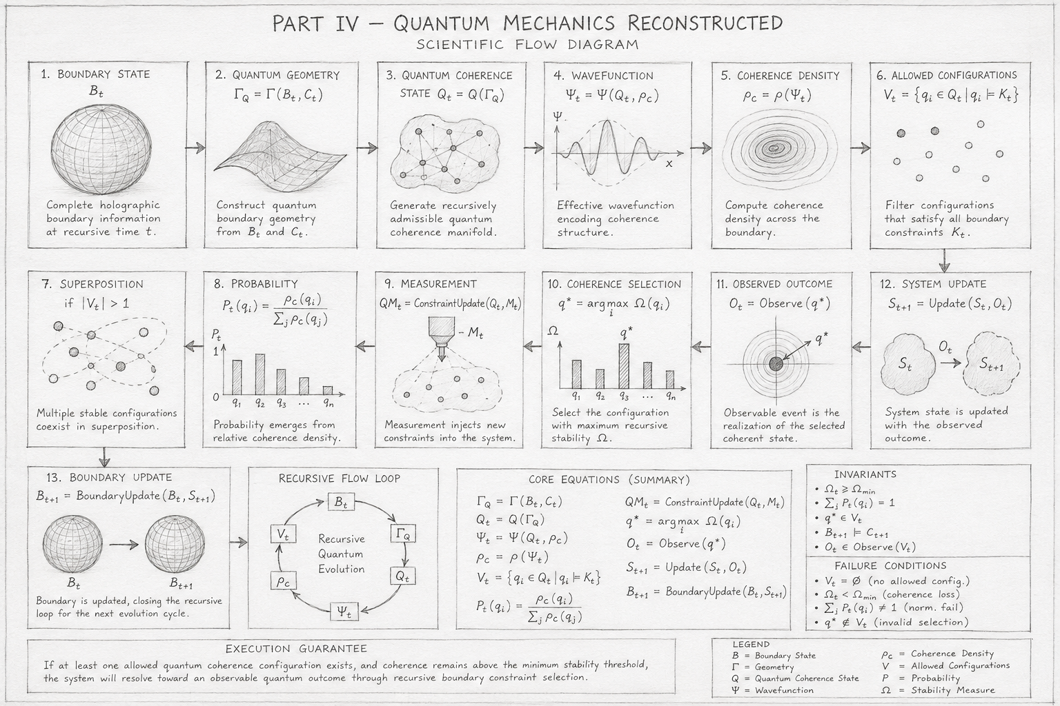
PART IV — Quantum Mechanics Reconstructed

Quantum mechanics has long been regarded as the most successful yet conceptually mysterious theory ever developed. Its mathematical framework predicts experimental observations with extraordinary precision, yet many of its central concepts—including wavefunction collapse, superposition, quantum probability, entanglement, and measurement—remain subjects of philosophical debate. The traditional formalism describes what quantum systems do with exceptional accuracy, but offers comparatively little consensus regarding why these behaviours arise at the deepest structural level.

Within the Holographic Space-Time (HST) framework, this situation is approached from an entirely different perspective. Rather than treating quantum mechanics as a collection of fundamentally probabilistic laws acting upon isolated particles, HST reconstructs quantum behaviour as the natural consequence of recursive boundary coherence evolving within a globally connected geometric information structure.

This reconstruction does not reject the mathematical predictions of conventional quantum theory. Instead, it seeks to explain why those mathematical structures emerge in the first place. In HST, the familiar equations of quantum mechanics become effective descriptions of a deeper coherence geometry governed by recursive constraint propagation rather than intrinsic randomness.

The standard interpretation introduces several conceptual assumptions that remain difficult to reconcile with classical intuition:

Although these ideas successfully reproduce experiments, they leave unanswered questions regarding the physical mechanisms that generate them.

HST proposes that many of these apparent mysteries arise because conventional quantum mechanics describes observable projections rather than the deeper recursive geometry from which those observations emerge.

Instead of beginning with particles and wavefunctions, HST begins with:

Observable quantum behaviour then emerges naturally from these deeper organisational principles.

Earlier parts of HST have progressively redefined the foundations of physics.

Matter is no longer viewed as collections of independent point particles.

Instead, stable objects become persistent recursive coherence structures embedded within boundary geometry.

Likewise,

fields become coherence gradients,

mass becomes stable curvature,

energy becomes recursive update capacity,

electromagnetism becomes boundary tension,

and spacetime itself becomes a projection of evolving holographic boundaries.

Part IV extends this reconstruction into quantum mechanics by asking a fundamental question:

This shift replaces object-based ontology with coherence-based ontology.

The central hypothesis of Part IV is that every observable quantum phenomenon arises from the recursive evolution of boundary coherence.

Instead of describing particles by isolated wavefunctions,

HST describes evolving coherence manifolds.

Instead of probability amplitudes,

HST describes recursive stability densities.

Instead of random collapse,

HST describes coherence selection.

Instead of discontinuous state reduction,

HST describes recursive constraint resolution.

In this framework, quantum behaviour is not fundamentally random.

Rather, apparent randomness reflects incomplete knowledge of the underlying recursive coherence landscape.

Perhaps the greatest conceptual change introduced by HST concerns measurement.

Traditional quantum mechanics often treats measurement as a fundamentally separate physical process that forces a wavefunction into a single outcome.

HST instead models measurement as an interaction between recursive coherence structures.

Observation introduces additional boundary constraints.

These constraints modify the available stable coherence configurations.

The system then recursively converges toward a new stable boundary solution.

No special collapse mechanism is required.

Measurement becomes another example of recursive boundary evolution.

Superposition has historically been interpreted as a particle simultaneously existing in many possible states.

Within HST this picture changes considerably.

A superposition represents multiple recursively consistent coherence pathways that remain simultaneously compatible with existing boundary constraints.

Prior to interaction, several coherence configurations possess comparable stability.

Measurement introduces new constraints.

Recursive selection gradually eliminates unstable branches while preserving the most coherent solution.

Thus superposition becomes a geometric property of recursive coherence rather than a paradoxical physical duplication of matter.

Quantum probabilities emerge naturally within HST without requiring fundamentally random physical laws.

Each possible system configuration possesses a corresponding coherence density.

Configurations exhibiting stronger recursive stability occupy larger regions of coherent solution space.

The likelihood of observing a given outcome reflects the relative stability of competing coherence structures rather than intrinsic randomness.

The familiar statistical behaviour described by the Born Rule therefore appears as an emergent consequence of recursive boundary geometry rather than an independent axiom.

Entanglement has often been interpreted as implying instantaneous communication across arbitrary distances.

HST offers a different interpretation.

Entangled systems originate from a shared recursive coherence history.

Although spatial projections later appear separated, both systems remain components of a larger coherent boundary structure.

Changes observed during measurement do not require faster-than-light signalling.

Instead, both measurements reveal different projections of the same globally coherent recursive geometry.

Correlation reflects shared structure rather than transmitted information.

Within conventional quantum mechanics, the wavefunction occupies a central mathematical role.

HST interprets the wavefunction differently.

Rather than representing a physically real probability cloud, the wavefunction becomes an effective mathematical representation of boundary coherence distributions.

Its evolution tracks the recursive propagation of coherence through allowable geometric configurations.

The wavefunction therefore serves as a computational description of underlying coherence dynamics rather than the fundamental physical object itself.

The uncertainty principle also receives a structural reinterpretation.

Rather than representing a fundamental limit imposed by nature on simultaneous knowledge of complementary variables, HST views uncertainty as arising from finite boundary resolution.

Every observation samples only part of the recursive coherence structure.

Increasing resolution in one coherence direction necessarily reduces available coherence information in another.

The uncertainty relation therefore expresses a geometric information trade-off rather than an intrinsic indeterminacy of physical reality.

Throughout Part IV, quantum mechanics is reconstructed into a unified geometric language.

Wave behaviour,

particle behaviour,

interference,

spin,

tunnelling,

vacuum fluctuations,

quantum fields,

and measurement

are all interpreted as different manifestations of recursive coherence evolving across holographic boundary structures.

Rather than introducing separate mechanisms for each phenomenon, HST seeks a common underlying principle:

Recursive boundary stability determines observable physical behaviour.

This principle allows apparently disconnected quantum phenomena to be understood as different projections of the same recursive geometric dynamics.

Part IV builds directly upon every preceding section of the HST framework.

Part I established the recursive logical foundations required for stable information processing.

Part II introduced coherence geometry as the organisational substrate underlying observable structure.

Part III demonstrated how classical fields emerge from recursive boundary dynamics.

Part IV now extends these principles into the quantum domain, showing that quantum mechanics need not represent a fundamentally separate layer of physics. Instead, it is interpreted as the small-scale regime in which recursive coherence structures dominate observable behaviour.

The transition from classical physics to quantum mechanics therefore becomes continuous rather than discontinuous. Both arise from the same underlying recursive principles, differing primarily in the scale, stability, and resolution of the coherence structures involved.

The chapters that follow pursue several interconnected scientific goals:

Part IV represents one of the most significant conceptual transitions within the Holographic Space-Time framework. Rather than treating quantum mechanics as a domain governed by fundamentally different physical laws, it seeks to show that quantum behaviour is the natural consequence of recursive coherence evolving within holographically encoded boundary geometry.

The chapters that follow examine each major aspect of quantum theory—from interference and uncertainty to tunnelling, spin, entanglement, vacuum structure, and quantum fields—and reinterpret them through a common mathematical language of recursive stability, boundary constraints, and coherence evolution.

Together, they aim to demonstrate that the apparent mysteries of quantum mechanics can be understood not as violations of classical reasoning, but as the observable signatures of a deeper and more unified geometric order.

This Flow Algebra provides the formal execution model for Part IV — Quantum Mechanics Reconstructed within the Holographic Space-Time (HST) framework. Rather than treating quantum mechanics as a collection of independent postulates based upon probability amplitudes, wavefunction collapse, and fundamentally random behaviour, the flow reconstructs quantum phenomena as the recursive evolution of coherent boundary geometry.

The flow is intentionally written as an executable scientific specification rather than a symbolic derivation. Every stage represents a physically meaningful transformation of the system, beginning with the construction of boundary geometry and ending with the production of an observable quantum event. In doing so, the flow establishes a complete recursive pipeline that connects microscopic coherence structures with macroscopic measurement outcomes.

Unlike conventional formulations that begin with the Schrödinger equation or Hilbert space operators, this implementation begins with recursive boundary organisation. Observable quantum behaviour emerges only after coherence has propagated through successive stages of geometric constraint resolution.

The principal objective of this flow is to demonstrate that quantum mechanics can be reconstructed as a recursive boundary process.

Instead of assuming that particles inherently possess probabilistic behaviour, the flow proposes that apparent probabilities arise from competing stable coherence configurations embedded within holographic boundary geometry.

The execution sequence therefore answers a fundamental scientific question:

Every operation in the flow contributes to answering this question.

The execution begins by transforming the current boundary state,

\[ B_t \]

into a quantum boundary geometry,

\[ \Gamma_Q \]

This is not merely a coordinate transformation.

Instead, it represents the organisation of all recursively connected boundary information into a coherent geometric manifold capable of supporting quantum behaviour.

Within HST, geometry is never passive.

Geometry actively stores recursive information through curvature, constraint relationships and holographic encoding.

Consequently,

\[ \Gamma_Q \]

acts as the substrate upon which all subsequent quantum evolution occurs.

The flow therefore establishes geometry before introducing quantum states.

Once the quantum boundary geometry exists, the system generates

\[ Q_t \]

Unlike the conventional wavefunction,

\[ Q_t \]

is not a probability object.

Instead, it represents the collection of recursively stable coherence configurations that are currently compatible with the surrounding boundary geometry.

This distinction is important.

The coherence state describes structural organisation rather than probabilistic uncertainty.

Every allowed quantum configuration corresponds to a recursively stable region of boundary coherence.

Only after coherence has been established does the flow generate

\[ \Psi_t \]

Within this reconstruction, the wavefunction is treated as an effective mathematical representation of the underlying coherence distribution rather than the fundamental physical entity.

This stage therefore implements an important conceptual reversal.

Traditional quantum mechanics begins with

\[ \Psi \]

HST derives

from recursive coherence.

The wavefunction becomes an observable projection of deeper geometric organisation.

The next operation evaluates the coherence density

\[ \rho_C \]

This quantity measures how strongly recursive stability is concentrated throughout the boundary geometry.

Rather than representing particle density or probability density directly,

measures structural persistence.

Regions of high coherence density correspond to configurations that remain stable under recursive update.

Regions of low coherence density gradually disappear during later selection processes.

This density field becomes the foundation for every subsequent quantum prediction.

The flow next constructs the allowable solution space,

\[ V_t \]

Rather than permitting every mathematically conceivable configuration,

the recursive engine filters all possibilities through existing boundary constraints.

Only coherence configurations satisfying all recursive consistency conditions remain.

This process replaces arbitrary quantum state spaces with physically meaningful recursive solution manifolds.

Consequently,

the observable universe contains only recursively admissible coherence structures.

One of the most significant implementations within the flow concerns quantum superposition.

If multiple coherence configurations satisfy every boundary constraint,

the system retains them simultaneously.

Importantly,

the flow does not interpret this as multiple particles existing simultaneously.

Instead,

multiple recursively stable coherence pathways coexist within the solution manifold.

Each branch remains viable because none has yet violated recursive stability.

Superposition therefore becomes a property of geometric compatibility rather than physical duplication.

This implementation removes many of the conceptual paradoxes associated with conventional interpretations.

After constructing the complete coherence landscape,

the flow derives

\[ P_t \]

Unlike traditional quantum mechanics,

probability is not introduced as a fundamental axiom.

Instead,

probability emerges directly from the relative coherence density of competing recursive configurations.

Configurations occupying larger stable coherence regions naturally possess higher observational likelihood.

Thus statistical behaviour becomes an emergent property of recursive geometry.

No intrinsic randomness is required.

Measurement enters the flow only after the recursive coherence landscape has been established.

The measurement interaction,

\[ M_t \]

does not collapse a wavefunction.

Instead,

it introduces additional boundary constraints into the recursive system.

These new constraints alter the allowable coherence manifold.

The measurement process therefore becomes another recursive update rather than a fundamentally different physical law.

This implementation unifies observation with ordinary recursive evolution.

Following measurement,

the recursive engine searches for the most stable remaining configuration,

\[ q^{*} \]

This stage performs coherence optimisation.

Instead of selecting an outcome randomly,

the flow identifies the configuration possessing the greatest recursive stability,

\[ \Omega(q_i) \]

The observed state therefore corresponds to the most coherent surviving boundary solution.

Wavefunction collapse is replaced entirely by recursive coherence selection.

Once the optimal coherence configuration has been identified,

the system generates the observable outcome,

\[ O_t \]

Importantly,

the observation is not the cause of reality.

Rather,

it is the visible manifestation of the recursive coherence solution already determined by the boundary evolution.

Observation therefore reveals the selected configuration rather than creating it.

No physical observation is isolated.

Every observation modifies future coherence evolution.

The flow therefore updates the global recursive system,

\[ S_{t+1} \]

using the newly observed information.

This guarantees temporal continuity across recursive updates.

The quantum system retains memory of previous coherence evolution.

Finally,

the boundary itself is updated,

\[ B_{t+1} \]

This closes the recursive execution loop.

The newly evolved boundary becomes the starting point for the next quantum evolution cycle.

Quantum mechanics therefore becomes a continuously self-consistent recursive process rather than a sequence of isolated measurements.

This Flow Algebra introduces several important conceptual innovations that distinguish it from conventional quantum formulations.

It reconstructs:

Together, these components provide a unified execution framework in which all major quantum phenomena arise from the same recursive principles.

This flow forms the central execution engine for Part IV and connects naturally to every preceding part of the HST framework.

It inherits:

and extends them into the quantum domain without introducing fundamentally new physical laws.

Instead of separating classical and quantum physics into different conceptual frameworks, the flow demonstrates that both regimes can be described using the same recursive boundary mathematics.

Classical behaviour corresponds to highly stable, large-scale coherence structures, while quantum behaviour arises in regimes where multiple coherent configurations remain simultaneously compatible with boundary constraints.

The PART IV — Quantum Mechanics Reconstructed Flow Algebra is designed to be read as a recursive execution sequence rather than as a conventional mathematical derivation.

Unlike traditional presentations of quantum mechanics, which often begin with differential equations, operators, or probability amplitudes, this flow begins with the recursive organisation of boundary geometry. Each stage represents a logical transformation in the evolution of the system, where the output of one operation becomes the input to the next.

The flow should therefore be interpreted as a scientific execution model that describes how quantum phenomena emerge from recursive boundary coherence. Reading the flow from top to bottom follows the causal progression from an encoded boundary state to an observable quantum outcome and finally to an updated boundary ready for the next cycle of evolution.

At its highest level, the flow follows a simple recursive structure:

Each block is executed in sequence. No stage is independent; every operation depends on the recursive information produced by the previous stage.

The flow always begins with

\[ B_t \]

This symbol represents the complete holographically encoded boundary at recursive time $t$. It contains the current geometric, informational, and coherence state of the system.

You should think of $B_t$ as the "initial condition" for the entire quantum evolution. It is not merely a spatial surface but the complete recursive description from which all subsequent structures are derived.

Nothing in the flow can occur until this boundary state has been defined.

The first transformation,

\[ B_t\rightarrow\Gamma_Q \]

builds the quantum boundary geometry.

Here the boundary information is organised into a coherent geometric manifold. This geometry is not passive; it stores recursive constraints and determines which quantum configurations are physically admissible.

When reading this step, interpret it as the creation of the structural environment within which quantum behaviour can occur.

The geometry then produces

\[ Q_t \]

This is the complete quantum coherence state compatible with the current boundary geometry.

Unlike a classical particle state, $Q_t$ represents all recursively stable coherence configurations that satisfy the existing boundary constraints.

Read this stage as the generation of the quantum solution landscape rather than the creation of individual particles.

Next,

\[ Q_t\rightarrow\Psi_t \]

The flow derives the effective wavefunction from the underlying coherence state.

This is a key conceptual difference from conventional quantum mechanics. The wavefunction is not the starting point of the theory but an emergent mathematical representation of recursive coherence.

When reading this step, remember that the wavefunction describes the boundary organisation rather than creating it.

The flow then computes

\[ \rho_C \]

Coherence density measures the local stability of recursive structures throughout the boundary geometry.

Regions with higher coherence density correspond to configurations that are more likely to persist through subsequent recursive updates.

This stage prepares the information required for both probability estimation and coherence selection.

The next operation constructs the admissible solution set,

\[ V_t \]

Not every mathematically possible configuration is accepted. Instead, the recursive engine filters the available states according to boundary constraints.

Read this step as a constraint-solving process in which only geometrically consistent coherence configurations survive.

This ensures that every subsequent quantum event arises from a physically valid recursive solution.

If more than one admissible configuration remains,

\[ \left|V_t\right|>1 \]

the system enters a state of superposition.

Within HST, this does not imply that a particle simultaneously exists in multiple realities. Instead, several coherence pathways remain equally compatible with the current boundary constraints.

When reading this stage, interpret superposition as the coexistence of multiple stable geometric solutions awaiting further constraint resolution.

The probability distribution,

\[ P_t \]

is computed directly from the coherence density.

The flow does not introduce probability as a fundamental law. Instead, probability reflects the relative stability of competing coherence configurations.

When reading this stage, understand that statistical behaviour emerges naturally from recursive geometry rather than from intrinsic randomness.

Measurement enters only after the coherence landscape has been established.

The interaction,

\[ M_t \]

introduces new boundary constraints.

Rather than collapsing a wavefunction, the measurement modifies the recursive solution space.

Read this stage as a geometric update to the boundary rather than as a mysterious external intervention.

The recursive engine then selects

\[ q^{*}=\operatorname*{arg\,max}_{q_i}\Omega(q_i) \]

the configuration with the greatest recursive stability.

This replaces the conventional concept of wavefunction collapse.

When reading this step, think of the system as performing an optimisation over the remaining coherence configurations, choosing the one that best satisfies all recursive constraints.

The selected configuration becomes

\[ O_t \]

Observation does not create reality; it reveals the stable coherence solution determined by the recursive process.

Read this stage as the appearance of an observable event resulting from the prior evolution of the coherence landscape.

Finally, the observed outcome updates the system state,

\[ S_{t+1} \]

which in turn updates the boundary,

\[ B_{t+1} \]

This closes the recursive loop.

The newly updated boundary becomes the starting point for the next execution cycle, ensuring that quantum evolution is continuous and self-consistent across time.

The Invariants define conditions that must remain true throughout execution. They are not additional calculations but scientific guarantees of consistency.

For example:

\[ \Omega_t\geq\Omega_{\min} \]

ensures that coherence remains sufficiently stable for the recursive process to continue.

Similarly,

\[ \sum_i P_t(q_i)=1 \]

guarantees that the emergent probability distribution is properly normalised.

These invariants should be read as conservation principles that preserve the physical validity of the reconstruction.

The Failure Conditions describe situations in which the recursive execution cannot proceed.

Examples include:

In physical terms, these conditions indicate that the current boundary state cannot support a consistent quantum evolution without first being redefined or stabilised.

The final section of the flow is the Execution Guarantee. This summarises the central promise of the reconstruction:

If at least one recursively stable quantum configuration exists and coherence remains above the minimum stability threshold, the recursive boundary dynamics will always converge to a physically observable quantum outcome.

This statement encapsulates the philosophy of the HST approach. Quantum behaviour is not governed by arbitrary collapse or intrinsic randomness but by the recursive evolution and selection of coherent boundary structures.

This flow should be read as the natural continuation of the earlier HST framework:

Accordingly, the flow is not a replacement for earlier chapters but an extension of them into the quantum regime.

When read as a whole, this Flow Algebra describes a complete recursive execution cycle:

Viewed in this way, the flow is more than a sequence of symbols—it is a complete geometric execution model that reconstructs quantum mechanics as the recursive evolution of holographically encoded boundary coherence.

It provides a unified language in which superposition, probability, measurement, and observation are all understood as successive stages of one continuous recursive process.

The scientific pencil diagram for Part IV — Quantum Mechanics Reconstructed presents the complete recursive execution architecture of quantum mechanics within the Holographic Space-Time (HST) framework. Rather than illustrating isolated quantum phenomena, the diagram visualises a continuous information-processing cycle in which observable quantum behaviour emerges from recursively evolving boundary coherence.

The figure should not be interpreted as a conventional quantum circuit or a particle trajectory. Instead, it is a recursive systems diagram, where each panel represents a well-defined stage in the evolution of holographically encoded boundary information. Read from left to right and top to bottom, the diagram follows the causal progression from an initial boundary state, through coherence formation and quantum state evolution, to observation and recursive boundary renewal.

Collectively, the thirteen stages demonstrate how geometry, coherence, probability, measurement, and observation arise as successive transformations within a single recursive framework.

The first panel depicts a holographic sphere representing the recursive boundary state,

\[ B_t \]

This sphere symbolises the complete information boundary at recursive time $t$. Every subsequent physical quantity shown in the diagram originates from this boundary. Unlike a simple spatial surface, $B_t$ contains the encoded curvature, coherence, recursive memory, and constraint information necessary to determine the system's future evolution.

The spherical representation emphasises that the boundary is a closed, self-consistent information manifold rather than an open geometric surface.

The second panel transforms the boundary into a curved geometric surface,

\[ \Gamma_Q=\Gamma(B_t,C_t) \]

The mesh illustrates the emergence of quantum geometry from the interaction between the boundary state and the coherence field. The curvature of the surface indicates that geometry is an active participant in recursive information processing rather than a passive background.

Within HST, this panel establishes the structural environment in which quantum coherence can exist.

The third panel replaces the smooth geometric surface with a network of interconnected nodes,

\[ Q_t=Q(\Gamma_Q) \]

These nodes represent recursively stable coherence configurations distributed across the quantum manifold. The connecting links illustrate that quantum states are not isolated entities but parts of an interconnected coherence network.

The diagram therefore shifts the interpretation of quantum states from point-like particles to recursively coupled regions of stable boundary organisation.

The fourth panel introduces the familiar sinusoidal wave,

\[ \Psi_t=\Psi(Q_t,\rho_C) \]

Within the HST reconstruction, the wave is not presented as the fundamental physical object. Instead, it serves as the observable mathematical representation of the underlying coherence structure generated in the previous stage.

The coordinate axes emphasise that the wavefunction is an effective projection of recursive coherence rather than an independent physical field.

The fifth panel depicts a series of concentric contours converging towards a central peak,

\[ \rho_C=\rho(\Psi_t) \]

These contours represent the spatial distribution of recursive stability. Regions of tightly packed contours correspond to high coherence density, indicating configurations that remain stable under recursive evolution.

Rather than representing matter density, the figure visualises the concentration of recursive coherence throughout the boundary geometry.

The sixth panel shows a collection of candidate quantum configurations,

\[ V_t=\{\,q_i\in Q_t\mid q_i\models K_t\,\} \]

Filled and unfilled circles illustrate the distinction between recursively admissible and excluded configurations. The filtering process symbolises the application of boundary constraints, ensuring that only coherence states satisfying all recursive conditions remain available for future evolution.

This panel demonstrates that quantum solution spaces are not arbitrary but are constrained by the underlying geometry.

The seventh panel depicts multiple configurations linked by overlapping dashed trajectories.

The condition,

\[ \left|V_t\right|>1 \]

indicates that more than one recursively stable configuration remains simultaneously viable.

The dashed loops illustrate coexistence rather than motion. Superposition is therefore represented as the simultaneous availability of multiple stable coherence pathways, each satisfying the current boundary constraints.

This interpretation differs fundamentally from picturing a particle existing in multiple places at once.

The eighth panel introduces a histogram representing the probability distribution,

\[ P_t(q_i)=\frac{\rho_C(q_i)}{\sum_j \rho_C(q_j)} \]

The differing column heights demonstrate that probabilities emerge from relative coherence densities. Taller columns correspond to configurations occupying larger regions of recursive stability.

The diagram therefore illustrates that probability is derived from geometry rather than introduced as an independent axiom.

The ninth panel shows a measurement device projecting new constraints onto the coherence manifold,$$QM_t=\mathrm{ConstraintUpdate}(Q_t,M_t).$$

\[ QM_t=\operatorname{ConstraintUpdate}(Q_t,M_t) \]

Rather than collapsing the wavefunction, the measuring apparatus modifies the boundary constraints governing the recursive system.

The scattered circles beneath the detector indicate that the available coherence configurations are reorganised by measurement rather than destroyed.

This visualisation reinforces the HST interpretation of observation as recursive constraint updating.

The tenth panel presents a stability graph in which one configuration possesses the highest coherence value,

\[ q^{*}=\operatorname*{arg\,max}_{q_i}\Omega(q_i) \]

The tallest column represents the recursively preferred solution. Selection occurs through optimisation of recursive stability rather than through random collapse.

This panel is central to the reconstruction, illustrating that observable outcomes emerge from maximising coherence within the constrained solution space.

The eleventh panel displays a target-like structure centred on the selected configuration,

\[ O_t=\operatorname{Observe}(q^{*}) \]

The concentric rings symbolise the projection of the selected coherence state into observable physical reality.

The diagram emphasises that observation reveals the outcome of recursive selection; it does not create the underlying state.

The twelfth panel illustrates the transition

\[ S_{t+1}=\operatorname{Update}(S_t,O_t) \]

A cloud-like representation of the system evolves into a new recursive state after incorporating the observed information. This panel demonstrates that every observation modifies the future evolution of the recursive system.

No observation is isolated; each contributes to the ongoing development of the coherence landscape.

The thirteenth panel returns to the holographic sphere,

\[ B_{t+1}=\operatorname{BoundaryUpdate}(B_t,S_{t+1}) \]

Two successive boundary states are shown, connected by an update arrow. This final stage closes the recursive loop, indicating that the updated boundary becomes the starting point for the next execution cycle.

The circular structure of the diagram reflects the self-consistent nature of recursive evolution.

The central recursive flow loop summarises the complete execution sequence:

\[ B_t\rightarrow\Gamma_Q\rightarrow Q_t\rightarrow\Psi_t\rightarrow\rho_C\rightarrow V_t\rightarrow q^{*}\rightarrow O_t\rightarrow S_{t+1}\rightarrow B_{t+1} \]

Unlike a linear algorithm, this loop demonstrates that quantum mechanics is an ongoing recursive process. Every completed observation generates the boundary conditions required for the next cycle of quantum evolution.

The lower central section gathers together the principal mathematical expressions used throughout the diagram.

These equations define:

Their placement illustrates that every graphical component corresponds directly to a formal mathematical operation within the HST framework.

The right-hand panels define the conditions under which recursive execution remains valid.

The Invariants express conservation principles that must always hold:

Beneath these, the Failure Conditions identify situations in which recursive execution cannot continue, including loss of coherence, absence of admissible configurations, invalid probability normalisation, or incoherent state selection.

Together, these sections distinguish the HST Flow Algebra from a descriptive diagram by specifying explicit mathematical conditions for successful execution.

Viewed as a whole, the diagram presents quantum mechanics as a continuous recursive information process rather than a sequence of isolated physical events. Geometry generates coherence, coherence gives rise to quantum states, quantum states define wavefunctions, coherence density determines probabilities, measurement introduces new constraints, recursive optimisation selects the most stable configuration, and observation updates the system before the boundary is regenerated.

This closed recursive architecture replaces the traditional picture of discontinuous wavefunction collapse with one of continuous coherence evolution. Every stage is mathematically connected to the next, and every observable quantum event is interpreted as the natural consequence of recursive boundary dynamics.

Within the broader Holographic Space-Time framework, this diagram therefore serves as the visual synthesis of Part IV — Quantum Mechanics Reconstructed, demonstrating how quantum behaviour can be understood as the emergent manifestation of recursively evolving holographic boundary coherence.

The PART IV — Quantum Mechanics Reconstructed Flow Algebra is constructed as a deterministic recursive execution framework in which every computational stage follows directly from the previous boundary state. Execution begins with the holographically encoded boundary $B_t$, constructs the corresponding quantum coherence geometry, generates the admissible quantum state manifold, evaluates coherence density, resolves recursively stable configurations, applies measurement as boundary constraint injection, and produces an observable quantum outcome before recursively updating the boundary for the next execution cycle.

Execution is guaranteed whenever the recursive boundary contains at least one physically admissible coherence configuration and all recursive stability conditions remain satisfied throughout the computation.

The flow executes successfully if and only if the following conditions hold:

\[ B_t\neq\varnothing \]

\[ \Gamma_Q\neq\varnothing \]

\[ Q_t\neq\varnothing \]

\[ V_t\neq\varnothing \]

\[ \Omega_t\geq\Omega_{\min} \]

\[ \sum_i P_t(q_i)=1 \]

\[ q^{*}\in V_t \]

Under these conditions, the recursive execution always converges to a physically admissible observable state,

\[ O_t=\operatorname{Observe}(q^{*}) \]

followed by the recursive system update,

\[ S_{t+1}=\operatorname{Update}(S_t,O_t) \]

and boundary renewal,

\[ B_{t+1}=\operatorname{BoundaryUpdate}(B_t,S_{t+1}) \]

The Flow Algebra guarantees that every successful execution completes the full recursive cycle:

\[ B_t\rightarrow\Gamma_Q\rightarrow Q_t\rightarrow\Psi_t\rightarrow\rho_C\rightarrow V_t\rightarrow P_t\rightarrow QM_t\rightarrow q^{*}\rightarrow O_t\rightarrow S_{t+1}\rightarrow B_{t+1} \]

No stage exists in isolation. Every output is uniquely determined by the recursive state produced by the preceding stage, ensuring continuity across the complete quantum evolution.

The Flow Algebra guarantees that:

Accordingly, all observable quantum behaviour is interpreted as the consequence of recursive boundary evolution.

Provided that

\[ \Omega_t\geq\Omega_{\min} \]

the recursive coherence manifold remains structurally stable throughout execution.

If multiple admissible configurations exist,

\[ \left|V_t\right|>1 \]

the system preserves them as a coherent superposition until additional boundary constraints are introduced. Recursive optimisation then selects

\[ q^{*}=\operatorname*{arg\,max}_{q_i}\Omega(q_i) \]

ensuring that the observable configuration always corresponds to the maximum recursively stable solution.

The recursive boundary remains mathematically self-consistent throughout execution.

Each completed quantum evolution satisfies

\[ B_{t+1}\models C_{t+1} \]

ensuring that every updated boundary preserves the coherence relationships required for future recursive evolution.

Consequently, no recursive information is discarded; it is reorganised into a new holographically encoded boundary state.

This ordering establishes a unified causal structure in which every observable quantum event arises from the recursive evolution of holographically encoded boundary coherence.