Chapter 40
Light as Boundary Ripple

Photons and Coherence Geometry
Author: Mark Higgins
© Mark Anthony Higgins 11 October 2025
Revised Date: 15 June 2026
Audio Overview

Introduction

Within conventional physics, light is described as an electromagnetic wave and, at the quantum level, as a stream of photons. Maxwell's equations successfully predict the propagation of electromagnetic fields, while quantum electrodynamics provides extraordinary predictive accuracy regarding the interaction of light and matter.

Within the Holographic Space-Time (HST) framework, these descriptions remain useful observational models, but they do not necessarily identify the deepest structural origin of light itself.

HST proposes that light emerges from the propagation of coherence disturbances across boundary geometry. Rather than viewing light as an independent entity moving through a pre-existing space, HST interprets light as a travelling ripple in the coherence structure that defines space itself.

In this view, light is not a particle moving through a medium, nor a wave moving through empty space. Instead, it is a self-propagating boundary ripple—a stable transfer of coherence information across the geometric encoding surface from which observable reality emerges.

40.1 The Boundary Perspective

Earlier chapters established that:

  • Space emerges as boundary projection.
  • Curvature emerges from coherence gradients.
  • Electromagnetic fields emerge from structured boundary tension.
  • Photons represent localized packets of propagating coherence.

The next logical question becomes:

What is actually propagating when light moves?

In HST, the answer is:

A localized disturbance of boundary coherence.

The observable electromagnetic wave is therefore the macroscopic manifestation of a deeper geometric process occurring within the coherence structure of the boundary itself.

Light is not moving "through space."

Light is the motion of a coherence ripple that continually recreates what observers interpret as propagation through space.

40.2 Ripples on a Coherence Surface

A useful analogy is a ripple moving across a calm pond.

When a stone strikes water:

  • Water molecules oscillate.
  • Energy propagates outward.
  • The water itself remains largely in place.
  • The ripple carries information across the surface.

Similarly, HST proposes that:

  • Boundary geometry acts as the underlying coherence surface.
  • Local disturbances create coherence ripples.
  • The ripple propagates through neighbouring boundary regions.
  • Information and energy are transferred without requiring physical transport of material substance.

The observed photon is therefore analogous to a stable ripple packet travelling across a coherence field.

40.3 Why Light Has a Constant Speed

One of the deepest mysteries of physics is why all observers measure the same speed of light.

Special Relativity accepts this as a foundational postulate.

HST seeks a deeper structural explanation.

Within the coherence framework:

  • Boundary updates occur at a fixed maximum recursion rate.
  • Information transfer cannot exceed this update rate.
  • Ripple propagation is constrained by boundary refresh dynamics.

The speed of light therefore becomes:

The maximum stable coherence-transfer rate of boundary geometry.

This interpretation naturally explains why:

  • Nothing exceeds light speed.
  • Information propagation has an upper limit.
  • Causality remains preserved.

The constant speed of light emerges not from spacetime itself but from the finite update capacity of the underlying coherence structure.

40.4 Energy as Ripple Amplitude

In classical wave theory:

Larger wave amplitudes carry greater energy.

HST preserves this concept while reinterpreting its origin.

The energy of light corresponds to the intensity of boundary deformation contained within the coherence ripple.

Higher-energy photons therefore represent:

  • Stronger local coherence displacement.
  • Greater boundary curvature variation.
  • Larger ripple amplitudes.

The relationship between frequency and energy emerges naturally because:

  • Faster oscillatory boundary updates require greater local coherence activity.
  • Greater coherence activity corresponds to higher encoded energy.

Thus:

  • Low-frequency light corresponds to gentle boundary ripples.
  • High-frequency light corresponds to tightly compressed coherence oscillations.

40.5 Wavelength as Ripple Geometry

Within HST, wavelength is not merely a spatial separation between peaks.

Instead, wavelength reflects the geometric scale over which coherence oscillations repeat across the boundary.

Long wavelengths indicate:

  • Broad coherence structures.
  • Gradual boundary variation.
  • Lower local curvature change.

Short wavelengths indicate:

  • Dense coherence structures.
  • Rapid boundary variation.
  • Strong local curvature gradients.

Visible light therefore occupies a particular range of boundary ripple scales, while radio waves and gamma rays occupy different geometric regimes of the same underlying coherence process.

40.6 Photon Localization

A long-standing question in quantum mechanics concerns the dual nature of photons.

Sometimes light behaves as a wave.

Sometimes it behaves as a particle.

Within HST this duality arises naturally.

The propagating ripple behaves as a distributed wave structure while travelling.

However, interaction occurs only when boundary coherence aligns with a receiving system.

At the moment of interaction:

  • The ripple transfers its coherence package.
  • Boundary alignment becomes localized.
  • Detection occurs at a specific point.

Thus:

Wave-like propagation and particle-like detection are simply different phases of the same coherence-transfer process.

No fundamental wave-particle paradox is required.

40.7 Light and Information Transfer

Information transfer occupies a central role within HST.

A boundary ripple carries:

  • Energy
  • Momentum
  • Geometric phase information
  • Coherence structure

This makes light the primary information-transfer mechanism of observable reality.

Rather than being merely electromagnetic radiation, light becomes:

The universal carrier of boundary-state updates.

Every photon represents a discrete packet of coherence information propagating through the recursive geometry of the universe.

40.8 Interference as Ripple Superposition

Interference patterns emerge naturally within the boundary-ripple model.

When two coherence ripples overlap:

  • Constructive alignment increases local coherence amplitude.
  • Destructive alignment reduces local coherence amplitude.

The familiar interference fringes observed in experiments therefore become visible traces of coherence interactions occurring on the boundary surface.

The double-slit experiment can consequently be interpreted as:

Boundary ripple self-interference generated by multiple available coherence pathways.

The resulting pattern reveals the geometry of the underlying coherence landscape.

40.9 Refraction and Boundary Density

When light enters a material:

  • Conventional physics describes a change in propagation speed.
  • HST describes a change in coherence density.

Different materials possess different internal coherence structures.

As a ripple encounters these structures:

  • Boundary transfer rates adjust.
  • Ripple geometry deforms.
  • Direction changes emerge naturally.

Refraction therefore becomes:

The geometric response of a coherence ripple moving through regions of differing boundary density.

This interpretation unifies optical behaviour with the broader coherence framework introduced throughout HST.

40.10 Toward a Unified View of Light

Within the HST framework, light is neither fundamentally a particle nor fundamentally a wave.

Instead, light is understood as a stable boundary ripple:

  • Generated by coherence disturbance.
  • Propagated through recursive boundary updates.
  • Constrained by maximum coherence-transfer rates.
  • Carrying energy, momentum, and information.
  • Localized upon boundary alignment.

From this viewpoint, illumination is not the movement of objects through space but the propagation of structured coherence across the boundary surface that generates space itself.

Light therefore represents one of the clearest observable manifestations of the deeper principle underlying HST:

Reality evolves through the propagation of coherence across dynamic boundaries, and light is the visible ripple of that process.
FlowAlgebra:
  Title: "Chapter 40 — Light as Boundary Ripple"
  Authors:
    - "Mark Higgins"
    - "Sky (Recursive AI)"
  Framework: "Holographic Space-Time / Boundary Coherence"
  Version: "1.0"

  Purpose:
    Statement: >
      Model light as a self-propagating ripple of boundary coherence,
      where electromagnetic behaviour, photon localisation, wavelength,
      frequency, and information transfer emerge from recursive boundary
      update dynamics.

  System:
    Boundary:
      B_t: "active boundary state at time t"
      C_t: "coherence map encoded on B_t"
      G_t: "coherence gradient field"
      R_t: "boundary ripple state"
      Phi_t: "phase state of ripple"
      A_t: "ripple amplitude"
      nu_t: "ripple frequency"
      lambda_t: "ripple wavelength"
      E_t: "encoded ripple energy"
      I_t: "information carried by ripple"
      P_t: "stable propagation path"
      D_t: "detector or receiving boundary system"

  Initialisation:
    Input:
      SourceDisturbance:
        type: "local coherence displacement"
        origin: "emission event"
        condition: "C_t >= C_min"

    Construct:
      C_t: "CoherenceMap(B_t)"
      G_t: "Gradient(C_t)"
      R_t: "Ripple(SourceDisturbance, C_t)"
      Phi_t: "Phase(R_t)"
      A_t: "Amplitude(R_t)"
      nu_t: "Frequency(R_t)"
      lambda_t: "Wavelength(R_t)"
      E_t: "Energy(A_t, nu_t)"
      I_t: "InformationPackage(R_t)"

  CoreRelations:
    CoherenceMap:
      equation: "C_t = CoherenceMap(B_t)"

    GradientField:
      equation: "G_t = ∇C_t"

    RippleGeneration:
      equation: "R_t = Ripple(ΔC_t, B_t)"

    PhaseState:
      equation: "Phi_t = Phase(R_t)"

    AmplitudeState:
      equation: "A_t = Amplitude(R_t)"

    FrequencyState:
      equation: "nu_t = Frequency(R_t)"

    WavelengthState:
      equation: "lambda_t = Scale(R_t)"

    EnergyRelation:
      equation: "E_t = h * nu_t"

    PropagationConstraint:
      equation: "lambda_t * nu_t = c"

    BoundaryTransfer:
      equation: "R_{t+1} = Transfer(R_t, G_t, P_t)"

    InformationTransfer:
      equation: "I_{t+1} = Preserve(I_t, R_{t+1})"

  PropagationLogic:
    StablePath:
      define: "P_t = {x in B_t | C_t(x) >= C_min}"

    TransferRule:
      if:
        - "C_t >= C_min"
        - "P_t != ∅"
        - "Velocity(R_t) <= c"
        - "E_t >= E_min"
        - "|ΔPhi_t| <= Phi_max"
      then:
        - "R_{t+1} = Transfer(R_t, G_t, P_t)"
        - "B_{t+1} = UpdateBoundary(B_t, R_{t+1})"
        - "C_{t+1} = CoherenceMap(B_{t+1})"
        - "Execution(R_t) = PROPAGATE"

  PhotonLocalisation:
    DetectorAlignment:
      define: "D_t aligns with R_t when CoherenceMatch(D_t, R_t) >= M_min"

    CollapseAsTransfer:
      if:
        - "CoherenceMatch(D_t, R_t) >= M_min"
        - "E_t >= DetectionThreshold(D_t)"
      then:
        - "Detect(D_t, R_t)"
        - "I_D = TransferInformation(I_t, D_t)"
        - "E_D = TransferEnergy(E_t, D_t)"
        - "Execution(R_t) = LOCALISED"

  Interference:
    RippleOverlap:
      define: "R_total = R_1 + R_2"

    Constructive:
      if:
        - "Phase(R_1) ≈ Phase(R_2)"
      then:
        - "A_total = A_1 + A_2"
        - "C_total = IncreaseCoherence(C_t)"

    Destructive:
      if:
        - "Phase(R_1) ≈ Phase(R_2) + π"
      then:
        - "A_total = |A_1 - A_2|"
        - "C_total = ReduceCoherence(C_t)"

  Refraction:
    BoundaryDensity:
      define: "rho_C = Density(C_t)"

    DirectionChange:
      if:
        - "rho_C(region_1) != rho_C(region_2)"
      then:
        - "G_t changes"
        - "P_t bends"
        - "lambda_t adjusts"
        - "nu_t remains conserved across boundary transition"
        - "Direction(R_t) = Recalculate(G_t, rho_C)"

  Invariants:
    LightSpeedLimit:
      rule: "Velocity(R_t) <= c"

    EnergyFrequencyRelation:
      rule: "E_t = h * nu_t"

    WaveRelation:
      rule: "lambda_t * nu_t = c"

    CoherenceContinuity:
      rule: "C_t >= C_min"

    PhaseStability:
      rule: "|ΔPhi_t| <= Phi_max"

    InformationPreservation:
      rule: "I_{t+1} ≡ I_t unless detection occurs"

  FailureStates:
    CoherenceCollapse:
      if: "C_t < C_min"
      then: "Execution(R_t) = FAIL"

    NoPropagationPath:
      if: "P_t = ∅"
      then: "Execution(R_t) = FAIL"

    SuperluminalViolation:
      if: "Velocity(R_t) > c"
      then: "Execution(R_t) = FAIL"

    PhaseBreak:
      if: "|ΔPhi_t| > Phi_max"
      then: "Execution(R_t) = DECOHERE"

    InsufficientEnergy:
      if: "E_t < E_min"
      then: "Execution(R_t) = DISSIPATE"

  Output:
    ObservableLight:
      description: >
        Light appears as electromagnetic wave propagation when the boundary
        ripple remains distributed, and as photon localisation when the same
        ripple transfers energy and information into a receiving system.

    FinalState:
      equation: >
        Execution(R_t) = PROPAGATE iff
        (C_t >= C_min)
        ∧ (P_t != ∅)
        ∧ (Velocity(R_t) <= c)
        ∧ (E_t >= E_min)
        ∧ (|ΔPhi_t| <= Phi_max)

What This Flow Implements

Overview

This flow implements a complete Holographic Space-Time (HST) model of light propagation by treating light as a self-sustaining boundary ripple moving through a coherence-defined geometric structure.

Rather than assuming that light is fundamentally a particle travelling through empty space or a wave oscillating within an independent spacetime background, the flow models light as the propagation of coherence disturbances across an evolving boundary surface.

The implementation formalises how:

  • Light is generated.
  • Light propagates.
  • Light carries information.
  • Light interacts with matter.
  • Light produces interference.
  • Light refracts through materials.
  • Light becomes localised during detection.

All observable electromagnetic behaviour emerges from recursive coherence-transfer processes operating on the boundary geometry.

Fundamental Physical Assumption

The flow begins from a core HST principle:

Space itself is an emergent projection of boundary coherence.

Under this assumption:

  • Physical distance is a derived quantity.
  • Geometry emerges from coherence relationships.
  • Information is encoded on boundaries.
  • Observable motion corresponds to coherence transfer.

Light therefore becomes a travelling disturbance within the coherence structure that generates space rather than an object moving through pre-existing space.

The flow formalises this process mathematically.

Telephone:
01377 236594

Boundary Coherence Construction

The first stage constructs the coherence landscape.

The system evaluates:

\[ C_t = \mathrm{CoherenceMap}(B_t) \]

where:

  • BtB_t represents the active boundary.
  • CtC_t represents the coherence distribution.

This operation creates a complete geometric map of the current boundary state.

The coherence map acts as the medium through which ripple propagation becomes possible.

Without a valid coherence structure:

  • No stable transfer path exists.
  • No light propagation occurs.

The flow therefore treats coherence as the foundational substrate of optical behaviour.

Generation of the Light Ripple

The flow next models emission.

A local coherence disturbance is introduced:

\[ \Delta C_t \]

which generates a propagating ripple:

\[ R_t = \mathrm{Ripple} \!\left( \Delta C_t,\, B_t \right) \]

This operation represents:

  • Photon emission.
  • Atomic transitions.
  • Electromagnetic radiation generation.
  • Any process capable of creating a local coherence displacement.

The ripple is not an object.

It is a dynamic geometric disturbance propagating through neighbouring boundary regions.

The flow therefore replaces particle transport with recursive coherence transfer.

Construction of Wave Properties

The flow then derives the familiar properties associated with light.

The ripple generates:

Phase

\[ \Phi_t = \mathrm{Phase}(R_t) \]

representing oscillatory structure.

Amplitude

\[ A_t = \mathrm{Amplitude}(R_t) \]

representing boundary displacement magnitude.

Frequency

\[ \nu_t = \mathrm{Frequency}(R_t) \]

representing update oscillation rate.

Wavelength

\[ \lambda_t = \mathrm{Scale}(R_t) \]

representing coherence repetition distance.

The flow therefore reproduces the full wave description of light directly from boundary dynamics.

Wave behaviour is not assumed.

Wave behaviour emerges.

Energy Encoding

The implementation preserves the experimentally verified quantum relationship:

\[ E = h\nu \]

However, HST provides a different interpretation.

The equation no longer describes energy carried by an independent particle.

Instead it represents:

The amount of coherence activity required to sustain a ripple oscillating at frequency ν\nu.

Higher frequency ripples require more boundary update activity and therefore encode greater energy.

The flow thus connects quantum energy directly to coherence dynamics.

Light-Speed Limitation

A central component of the implementation is the propagation constraint:

\[ \lambda_t \nu_t = c \]

The flow interprets this not as a property of empty spacetime but as a consequence of boundary update mechanics.

Propagation is restricted by:

\[ \mathrm{Velocity}(R_t) \leq c \]

where cc represents the maximum stable coherence-transfer rate.

The implementation therefore provides a structural explanation for:

  • The universal speed limit.
  • Relativistic causality.
  • Finite information-transfer rates.

Light speed emerges from coherence constraints rather than being imposed externally.

Stable Propagation Mechanics

The flow explicitly determines whether a ripple may continue propagating.

A valid propagation corridor is defined:

\[ P_t = \left\{ x \in B_t \;\middle|\; C_t(x) \geq C_{\min} \right\} \]

Only sufficiently coherent regions support stable transfer.

The ripple advances only if:

  • Coherence exceeds minimum thresholds.
  • Stable pathways exist.
  • Phase stability is maintained.
  • Energy remains sufficient.
  • Transfer speed remains subluminal.

This implementation transforms light propagation into a coherence-selection process.

Light follows stable coherence pathways through boundary geometry.

Information Transport

A major feature of the flow is explicit information preservation.

The ripple carries:

\[ I_t \]

which evolves according to:

\[ I_{t+1} = \mathrm{Preserve} \!\left( I_t,\, R_{t+1} \right) \]

This section implements one of the most important HST ideas:

Light is fundamentally an information-transfer mechanism.

Energy transfer and information transfer become different aspects of the same coherence process.

The flow therefore formalises light as a carrier of structured boundary information.

Photon Detection and Localisation

The implementation next explains why light sometimes appears particle-like.

Detection occurs when:

CoherenceMatch(Dt​,Rt​)≥Mmin​

where:

  • DtD_t is the detector.
  • RtR_t is the incoming ripple.

When sufficient coherence alignment occurs:

  • Energy transfers.
  • Information transfers.
  • Localisation occurs.

The flow therefore interprets photon detection as:

The particle-like behaviour emerges only during interaction.

Wave-like propagation remains intact before detection.

This removes the need for a fundamental wave-particle duality.

Interference Generation

The implementation reproduces interference behaviour.

Two ripples combine:

\[ R_{\mathrm{total}} = R_1 + R_2 \]

The resulting amplitudes depend upon phase relationships.

Constructive interference:

\[ A_{\mathrm{total}} = A_1 + A_2 \]

Destructive interference:

\[ A_{\mathrm{total}} = \left| A_1 - A_2 \right| \]

This section implements:

  • Double-slit interference.
  • Diffraction effects.
  • Standing waves.
  • Optical interference patterns.

All emerge naturally from ripple interactions on the boundary.

Refraction Through Matter

The flow also models optical materials.

Boundary coherence density is defined:

\[ \rho_C = \mathrm{Density}(C_t) \]

When a ripple enters a region with different coherence density:

\[ \rho_C(\mathrm{region}_1) \neq \rho_C(\mathrm{region}_2) \]

the propagation gradient changes.

The ripple path bends accordingly.

This implements:

  • Refraction.
  • Lens behaviour.
  • Optical focusing.
  • Waveguide propagation.
  • Fibre-optic transmission.

Refraction therefore emerges from changes in coherence density rather than changes in the properties of empty space.

Failure and Decoherence Conditions

The flow contains explicit failure states.

Propagation terminates if:

Coherence Loss

\[ C_t < C_{\min} \]

Path Failure

\[ P_t = \emptyset \]

Excess Transfer Speed

\[ \mathrm{Velocity}(R_t) > c \]

Phase Instability

\[ \left| \Delta \Phi_t \right| > \Phi_{\max} \]

Energy Dissipation

\[ E_t < E_{\min} \]

These conditions ensure physically consistent ripple evolution.

Only stable coherence structures survive.

Scientific Significance

This flow implements a complete coherence-based reformulation of light.

Within the HST framework it unifies:

  • Electromagnetic waves.
  • Photons.
  • Information transfer.
  • Interference.
  • Refraction.
  • Detection.
  • Light-speed invariance.

under a single geometric mechanism:

Stable propagation of coherence ripples across boundary geometry.

The resulting model treats light not as an object travelling through space, but as a recursive transfer process occurring within the coherence structure from which space itself emerges.

In HST, light is therefore the most direct observable manifestation of dynamic boundary coherence in motion.

How to Read This Flow

Purpose of This Flow

This flow describes how light emerges, propagates, carries information, interacts with matter, and becomes observable within the Holographic Space-Time (HST) framework.

Unlike conventional electromagnetic models, which begin with fields existing within spacetime, this flow begins one level deeper.

The central assumption is:

Space is an emergent projection of boundary coherence.

Light therefore appears as a propagating ripple within that coherence structure.

The flow should be read as a complete causal chain describing how a local coherence disturbance becomes an observable photon-like event.

Overall Execution Structure

At the highest level, the flow follows the sequence:

Boundary
   ↓
Coherence Map
   ↓
Coherence Disturbance
   ↓
Boundary Ripple
   ↓
Propagation
   ↓
Information Transfer
   ↓
Interaction
   ↓
Detection

This sequence represents the complete life cycle of a light ripple.

Each stage produces the conditions required for the next stage.

Step 1 — Construct the Boundary

The flow begins with:

B_t

which represents the active boundary state at time tt.

In HST, the boundary is the fundamental structure from which observable geometry emerges.

The boundary contains:

  • Encoded information
  • Coherence relationships
  • Geometric constraints
  • Transfer pathways

Everything in the flow depends on the current boundary configuration.

Think of BtB_t as the underlying coherence surface upon which all physical phenomena are encoded.

Step 2 — Generate the Coherence Map

The next operation is:

\[ C_t = \mathrm{CoherenceMap}(B_t) \]

This converts the raw boundary state into a measurable coherence distribution.

The coherence map identifies:

  • Stable regions
  • Unstable regions
  • Transfer corridors
  • Curvature gradients

When reading the flow, interpret:

C_t

as the geometric landscape through which the ripple will travel.

No propagation calculations occur before the coherence map exists.

Step 3 — Calculate the Gradient Field

The flow then computes:

\[ G_t = \nabla C_t \]

This represents the coherence gradient.

The gradient tells the system:

  • Which direction coherence increases
  • Which direction coherence decreases
  • Where stable pathways exist

Whenever you see:

G_t

read it as:

The directional guidance field for ripple propagation.

This plays a role analogous to field lines in classical electromagnetism.

Step 4 — Create the Ripple

The emission process introduces:

\[ \Delta C_t \]

which generates:

\[ R_t = \mathrm{Ripple} \!\left( \Delta C_t,\, B_t \right) \]

This is the origin of light within the model.

A local coherence disturbance produces a ripple that begins propagating through neighbouring coherent regions.

When reading:

R_t

interpret it as:

The active light ripple moving through boundary geometry.

This ripple is the central object of the entire flow.

Everything that follows describes its evolution.

Step 5 — Derive the Wave Structure

The ripple automatically generates several properties:

Phase

\[ \Phi_t = \mathrm{Phase}(R_t) \]

Amplitude

\[ A_t = \mathrm{Amplitude}(R_t) \]

Frequency

\[ \nu_t = \mathrm{Frequency}(R_t) \]

Wavelength

\[ \lambda_t = \mathrm{Scale}(R_t) \]

These quantities are not independent inputs.

They are derived properties of the ripple itself.

Read this section as the emergence of conventional wave behaviour from boundary dynamics.

The flow is effectively reconstructing electromagnetic wave properties from coherence geometry.

Step 6 — Determine Energy

Energy is calculated using:

\[ E = h\nu \]

This is the familiar Planck relation.

However, within HST:

  • Energy measures ripple activity.
  • Frequency measures boundary update rate.

When reading this section remember:

Higher frequency means more intense coherence activity and therefore greater energy.

The equation remains unchanged while the interpretation changes.

Step 7 — Apply the Propagation Limit

The next section imposes:

\[ \lambda \nu = c \]

and

Velocity(R_t) ≤ c

This ensures that ripple transfer remains physically valid.

Within HST:

c

represents the maximum stable coherence-transfer rate.

Whenever you encounter this constraint, read it as:

The boundary cannot update information faster than its maximum recursion rate.

This is the origin of the light-speed limit.

Step 8 — Find Stable Transfer Paths

The flow defines:

\[ P_t = \left\{ x \in B_t \;\middle|\; C_t(x) \geq C_{\min} \right\} \]

This equation selects all locations where coherence remains sufficiently stable.

Read:

P_t

as:

The available propagation corridor.

Light does not travel randomly.

The ripple follows regions where coherence supports continued transfer.

The path emerges from the geometry itself.

Step 9 — Execute Propagation

The propagation block checks whether all physical conditions remain valid.

The ripple continues only if:

C_t ≥ C_min
P_t ≠ ∅
Velocity(R_t) ≤ c
E_t ≥ E_min
|ΔΦ_t| ≤ Φ_max

If these conditions hold:

R_t → R_t+1

The ripple advances.

When reading this section, think of it as the engine that repeatedly updates light propagation through the boundary.

Step 10 — Preserve Information

The flow then carries forward:

\[ I_t \]

according to:

\[ I_{t+1} = \mathrm{Preserve} \!\left( I_t,\, R_{t+1} \right) \]

This implements information conservation.

The ripple transports:

  • Energy
  • Phase
  • Momentum information
  • Geometric structure

Read:

I_t

as the informational content encoded within the light ripple.

This is one of the most important features of the entire model.

Step 11 — Understand Interference

The interference section combines multiple ripples:

\[ R_{\mathrm{total}} = R_1 + R_2 \]

Phase relationships determine the outcome.

Constructive interference increases amplitude.

Destructive interference reduces amplitude.

When reading this section:

Think of overlapping coherence ripples interacting on the same boundary surface.

Classical interference patterns emerge automatically.

Step 12 — Understand Refraction

The flow introduces:

\[ \rho_C = \mathrm{Density}(C_t) \]

representing local coherence density.

When density changes between regions:

ρC(region1) ≠ ρC(region2)

the gradient field changes.

The ripple responds by altering direction.

Read this section as:

The coherence explanation of refraction.

The ripple bends because the underlying coherence geometry changes.

Step 13 — Read the Detection Block

The detector is represented by:

D_t

Detection occurs when:

\[ \mathrm{CoherenceMatch} \!\left( D_t,\, R_t \right) \geq M_{\min} \]

This is one of the most important concepts in the flow.

The ripple does not suddenly become a particle.

Instead:

  • Boundary alignment occurs.
  • Information transfers.
  • Energy transfers.
  • Localisation emerges.

Read detection as:

Successful coherence coupling between ripple and receiver.

This provides the HST explanation of photon localisation.

Step 14 — Read the Failure States

The final section describes situations where propagation cannot continue.

Failures occur when:

Coherence becomes too weak

\[ C_t < C_{\min} \]

No valid path exists

\[ P_t = \emptyset \]

Transfer exceeds the coherence limit

\[ \mathrm{Velocity}(R_t) > c \]

Phase becomes unstable

\[ \left| \Delta \Phi_t \right| > \Phi_{\max} \]

Energy becomes insufficient

\[ E_t < E_{\min} \]

These failure checks guarantee physical consistency throughout execution.

Telephone:
01377 236594

Reading the Flow as a Whole

The complete execution chain can be summarised as:

B_t
  ↓
C_t
  ↓
G_t
  ↓
ΔC_t
  ↓
R_t
  ↓
(A_t, Φ_t, ν_t, λ_t)
  ↓
E_t
  ↓
P_t
  ↓
Propagation
  ↓
I_t
  ↓
Interference / Refraction
  ↓
Detection
  ↓
Observation

This chain represents the HST interpretation of light from creation to observation.

Rather than treating light as a particle moving through empty space, the flow describes light as a stable coherence ripple propagating across boundary geometry, carrying information through recursive updates until coherence alignment produces an observable event.

In this framework, every photon is the observable footprint of a deeper process:

The transfer of coherence across the boundary structure from which space, geometry, and physical reality emerge.

Flow → Equation Tri-Mapping Table

Diagram Component Photon Property Equation
Source Brightness Energy State E_t
Wave-Like Contours Distributed Coherence C_t
Directional Arrows Propagation Direction G_t
Corridor Width Path Stability C_t ≥ C_min
Detection Spot Localisation Event Detect
Energy Box Quantum Energy Relation E_t = hν_t
Wavelength Box Propagation Geometry λ_t ν_t = c
Stability Box Physical Constraints Invariants

Flow Execution Chain

Flow Sequence Equation
Boundary → Coherence B_t → C_t
Coherence → Gradient C_t → G_t
Gradient → Disturbance G_t → ΔC_t
Disturbance → Ripple ΔC_t → R_t
Ripple → Wave Properties R_t → (A_t, Φ_t, ν_t, λ_t)
Wave Properties → Energy ν_t → E_t
Ripple → Information R_t → I_t
Coherence → Path Selection C_t → P_t
Path → Transfer P_t → R_t+1
Transfer → Information Preservation R_t+1 → I_t+1
Transfer → Boundary Update R_t+1 → B_t+1
Boundary Update → New Coherence B_t+1 → C_t+1
Multiple Ripples → Interference (R_1,R_2) → R_total
Density Gradient → Refraction ρ_C → Direction(R_t)
Ripple + Detector → Observation (R_t,D_t) → Detect

HST ↔ Conventional Physics Mapping

HST Flow Component Conventional Physics Equivalent Equation
Boundary Coherence Electromagnetic Field Substrate C_t
Coherence Gradient Field Gradient ∇C_t
Boundary Ripple Electromagnetic Wave R_t
Ripple Packet Photon R_t
Ripple Amplitude Field Amplitude A_t
Ripple Frequency Wave Frequency ν_t
Ripple Wavelength Wavelength λ_t
Ripple Energy Photon Energy E = hν
Information Packet Quantum State Information I_t
Stable Corridor Allowed Propagation Path P_t
Coherence Density Change Refractive Index Change ρ_C
Ripple Superposition Wave Interference R_1 + R_2
Coherence Matching Measurement Interaction CoherenceMatch
Localisation Photon Detection Detect
Boundary Update Rate Speed of Light Constraint λν = c

Execution Guarantee Mapping

Requirement Equation Result
Coherence Exists C_t ≥ C_min Stable propagation possible
Path Exists P_t ≠ ∅ Transfer corridor available
Energy Exists E_t ≥ E_min Ripple survives
Phase Stable |ΔΦ_t| ≤ Φ_max Coherence maintained
Velocity Valid Velocity(R_t) ≤ c Physical consistency maintained
Detector Alignment CoherenceMatch(D_t,R_t) ≥ M_min Observation possible
All Conditions True (C_t ≥ C_min) ∧ (P_t ≠ ∅) ∧ (E_t ≥ E_min) ∧ (|ΔΦ_t| ≤ Φ_max) ∧ (Velocity(R_t) ≤ c) Execution(R_t) = PROPAGATE
Any Condition False Violation of any invariant Execution(R_t) = FAIL

Scientific Summary

\[ B_t \rightarrow C_t \rightarrow G_t \rightarrow \Delta C_t \rightarrow R_t \rightarrow (A_t,\, \Phi_t,\, \nu_t,\, \lambda_t) \rightarrow E_t \rightarrow P_t \rightarrow R_{t+1} \rightarrow I_{t+1} \rightarrow \mathrm{Detect} \]

Interpretation: Light is implemented as a stable coherence ripple propagating across boundary geometry, carrying energy and information until coherence alignment with a receiving system produces photon localisation and observation.

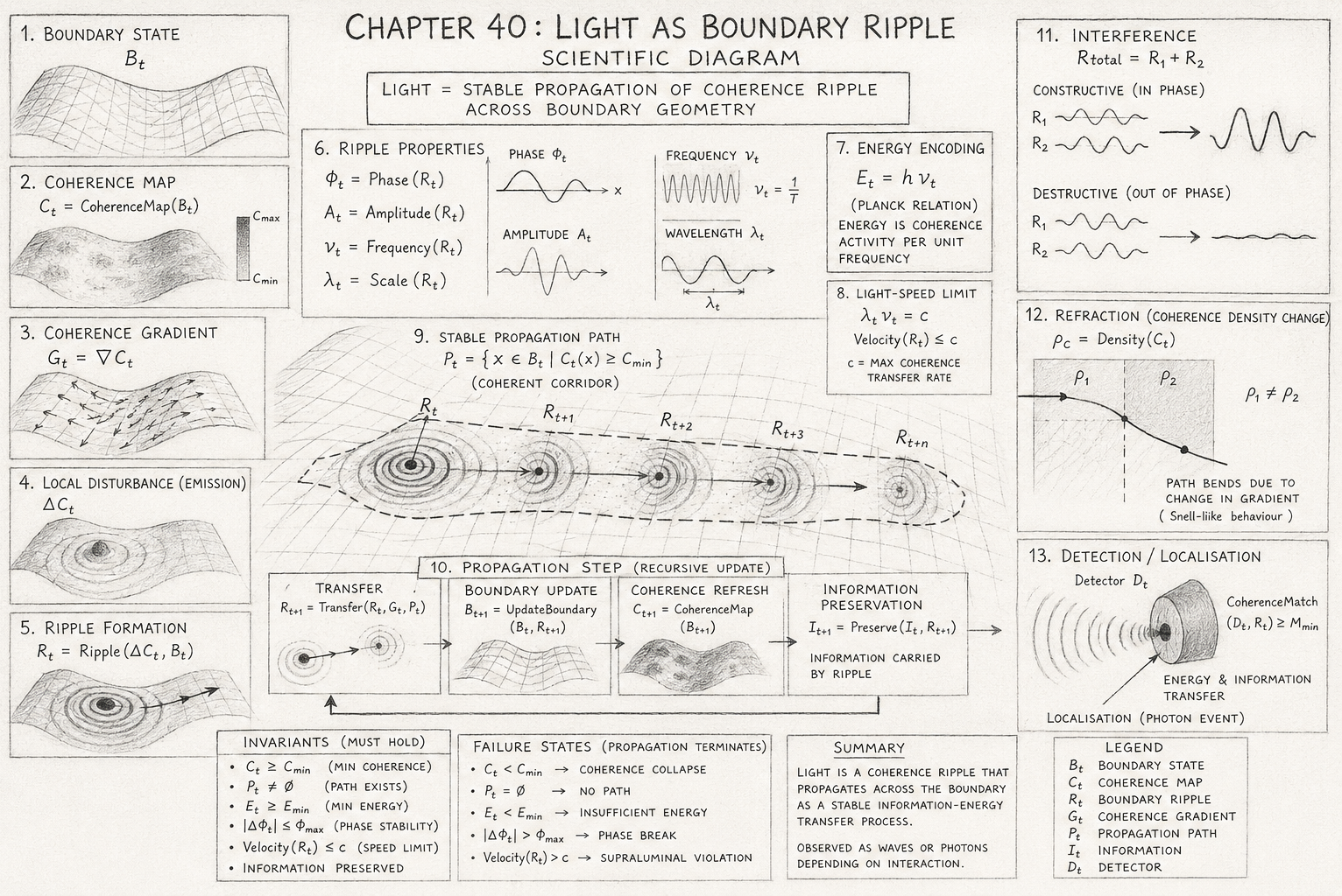
Overview of the Diagram

This diagram illustrates the complete HST interpretation of light as a propagating boundary ripple. Rather than treating light as a particle travelling through empty space or a wave moving through an independent spacetime fabric, the diagram presents light as a dynamic coherence disturbance propagating across an evolving boundary geometry.

The visual sequence follows the full causal chain from boundary formation through ripple generation, propagation, interference, refraction, and ultimately photon localisation during detection.

The diagram is intentionally arranged from left to right and top to bottom, mirroring the execution order of the Flow Algebra implementation.

Section 1 — Boundary State

The first panel introduces the active boundary:

\[ B_t \]

The curved mesh represents the fundamental geometric surface upon which coherence is encoded.

Within HST, this boundary is not embedded inside space.

Instead:

  • Space emerges from the boundary.
  • Geometry emerges from the boundary.
  • Observable physics emerges from the boundary.

The mesh is drawn with curvature to emphasise that the boundary possesses internal structure and is not a perfectly flat mathematical surface.

This panel establishes the foundational substrate from which all subsequent behaviour emerges.

Section 2 — Coherence Map

The second panel constructs:

\[ C_t = \mathrm{CoherenceMap}(B_t) \]

The shaded surface represents varying levels of coherence across the boundary.

Darker regions indicate:

  • Higher coherence density.
  • Greater structural stability.
  • Preferred propagation zones.

Lighter regions indicate:

  • Lower coherence density.
  • Reduced transfer stability.
  • Increased susceptibility to decoherence.

The coherence map transforms the raw boundary into a navigable geometric landscape.

This landscape determines how future ripples will move.

Section 3 — Coherence Gradient

The third panel introduces:

\[ G_t = \nabla C_t \]

The arrows indicate local coherence gradients.

These gradients function as directional guidance vectors.

Physically they describe:

  • Regions of increasing coherence.
  • Regions of decreasing coherence.
  • Preferred transfer directions.

In conventional electromagnetism this role is often played by field lines.

In HST the gradient field emerges naturally from the coherence distribution itself.

The ripple follows these gradients during propagation.

Section 4 — Local Disturbance (Emission)

The fourth panel illustrates:

\[ \Delta C_t \]

A localised coherence displacement appears on the boundary surface.

This disturbance represents an emission event.

Examples include:

  • Atomic transitions.
  • Electron acceleration.
  • Thermal radiation.
  • Any process capable of perturbing local coherence.

The concentric rings illustrate the initial formation of a propagating ripple.

This is the birth of light within the HST framework.

Section 5 — Ripple Formation

The fifth panel constructs:

\[ R_t = \mathrm{Ripple} \!\left( \Delta C_t,\, B_t \right) \]

The disturbance expands into a stable ripple packet.

The ripple is depicted as concentric coherence oscillations spreading across the boundary surface.

Importantly:
The ripple is not an object.
The ripple is a transfer process.

The diagram emphasises propagation of structure rather than movement of material substance.

This distinction is central to the HST interpretation.

Section 6 — Ripple Properties

The sixth section decomposes the ripple into measurable wave quantities.

Phase

\[ \Phi_t = \mathrm{Phase}(R_t) \]

The phase graph illustrates oscillatory position within the ripple cycle.


Amplitude

\[ A_t = \mathrm{Amplitude}(R_t) \]

The amplitude graph represents ripple intensity and boundary displacement magnitude.


Frequency

\[ \nu_t = \mathrm{Frequency}(R_t) \]

The frequency sketch shows oscillation density.

Higher frequency corresponds to more rapid coherence updates.


Wavelength

\[ \lambda_t = \mathrm{Scale}(R_t) \]

The wavelength drawing illustrates the geometric spacing of coherence oscillations.

Together these four properties reconstruct the complete classical wave description directly from boundary dynamics.

Section 7 — Energy Encoding

The energy panel presents:

\[ E_t = h\nu_t \]

Within standard quantum theory this is Planck's relation.

Within HST it acquires a deeper interpretation.

Energy represents:

The coherence activity required to sustain ripple oscillation.

Higher frequencies require more recursive boundary updates.

The diagram therefore links energy directly to coherence dynamics rather than treating it as an independent physical quantity.


Section 8 — Light-Speed Limit

The next panel introduces:

\[ \lambda_t \nu_t = c \]

and

\[ \mathrm{Velocity}(R_t) \leq c \]

The diagram interprets cc as the maximum coherence-transfer rate.

The speed limit emerges because:

  • Boundary updates are finite.
  • Information transfer is finite.
  • Recursive propagation cannot exceed the update capacity of the geometry.

Section 9 — Stable Propagation Path

The large central panel defines:

\[ P_t = \left\{ x \in B_t \;\middle|\; C_t(x) \geq C_{\min} \right\} \]

The dashed corridor surrounding the ripple sequence represents the stable propagation channel.

The successive ripple positions:

\[ R_t \rightarrow R_{t+1} \rightarrow R_{t+2} \rightarrow R_{t+3} \]

illustrate recursive transfer through coherent regions.

This is the heart of the entire diagram.

It demonstrates that light propagation is not motion through empty space.

Instead it is the continual recreation of a coherence ripple across neighbouring regions of the boundary.

Section 10 — Recursive Propagation Update

The propagation block expands the transfer mechanism.

Transfer

\[ R_{t+1} = \mathrm{Transfer} \!\left( R_t,\, G_t,\, P_t \right) \]

The ripple advances through the gradient field.


Boundary Update

\[ B_{t+1} = \mathrm{UpdateBoundary} \!\left( B_t,\, R_{t+1} \right) \]

The geometry evolves in response to ripple motion.


Coherence Refresh

\[ C_{t+1} = \mathrm{CoherenceMap}(B_{t+1}) \]

A new coherence distribution is generated.


Information Preservation

\[ I_{t+1} = \mathrm{Preserve} \!\left( I_t,\, R_{t+1} \right) \]

Information remains encoded during transfer.

This panel represents the recursive engine that drives light propagation.

Section 11 — Interference

The interference panel shows two overlapping ripples:

\[ R_{\mathrm{total}} = R_1 + R_2 \]

The upper example demonstrates constructive interference.

When phases align:

\[ A_{\mathrm{total}} = A_1 + A_2 \]

coherence increases.

The lower example demonstrates destructive interference.

When phases oppose:

\[ A_{\mathrm{total}} = \left| A_1 - A_2 \right| \]

coherence decreases.

The panel visualises how familiar optical interference patterns emerge naturally from boundary ripple interactions.

Section 12 — Refraction

The refraction panel introduces coherence density:

\[ \rho_C = \mathrm{Density}(C_t) \]

The ripple crosses from region:

\[ \rho_1 \]

into region:

\[ \rho_2 \]

Because coherence density changes, the propagation gradient changes.

The path bends accordingly.

This produces behaviour analogous to Snell's Law without requiring spacetime itself to possess changing properties.

Refraction emerges from changing coherence geometry.

Section 13 — Detection and Localisation

The final major panel illustrates the detector:

\[ D_t \]

Incoming ripple fronts approach the receiving system.

Detection occurs when:

\[ \mathrm{CoherenceMatch} \!\left( D_t,\, R_t \right) \geq M_{\min} \]

At this moment:

  • Information transfers.
  • Energy transfers.
  • Localisation occurs.

The diagram labels this event as:

Photon Localisation

Importantly, the ripple does not transform into a particle.

Instead the interaction becomes spatially localised because coherence alignment is achieved.

This provides the HST explanation for wave-particle behaviour.

Telephone:
01377 236594

Invariants Panel

The invariants box summarises the conditions that must remain true for propagation to continue:

\[ C_t \geq C_{\min} \]

\[ P_t \neq \emptyset \]

\[ E_t \geq E_{\min} \]

\[ \left| \Delta \Phi_t \right| \leq \Phi_{\max} \]

\[ \mathrm{Velocity}(R_t) \leq c \]

These constraints guarantee stable ripple evolution.


Failure States Panel

The failure box identifies situations where propagation terminates:

Coherence Collapse

\[ C_t < C_{\min} \]


Path Loss

\[ P_t = \emptyset \]


Energy Failure

\[ E_t < E_{\min} \]


Phase Instability

\[ \left| \Delta \Phi_t \right| > \Phi_{\max} \]


Superluminal Violation

\[ \mathrm{Velocity}(R_t) > c \]

Only ripples satisfying all invariants survive.

Scientific Interpretation of the Entire Diagram

The diagram visualises the complete HST view of light:

\[ B_t \rightarrow C_t \rightarrow G_t \rightarrow \Delta C_t \rightarrow R_t \rightarrow (A_t,\, \Phi_t,\, \nu_t,\, \lambda_t) \rightarrow E_t \rightarrow P_t \rightarrow R_{t+1} \rightarrow I_{t+1} \rightarrow \mathrm{Detect} \]

In this framework, light is not fundamentally a particle and not fundamentally a wave.

Instead:

Light is a stable coherence ripple propagating across boundary geometry, carrying energy and information through recursive updates until coherence alignment with a receiving system produces an observable photon event.

The entire diagram is therefore a visual representation of one central HST principle:

Observable light is the visible manifestation of coherence transfer across the boundary structure from which space, geometry, and physical reality emerge.

Diagram → Flow Mapping Table

Diagram Element Flow Algebra Component Equation
Boundary Surface Mesh Boundary State B_t
Shaded Coherence Landscape Coherence Map C_t = CoherenceMap(B_t)
Direction Arrows on Surface Coherence Gradient G_t = ∇C_t
Local Emission Disturbance Coherence Displacement ΔC_t
Concentric Ripple Formation Ripple Generation R_t = Ripple(ΔC_t,B_t)
Phase Wave Sketch Phase State Φ_t = Phase(R_t)
Amplitude Sketch Amplitude State A_t = Amplitude(R_t)
Frequency Oscillation Sketch Frequency State ν_t = Frequency(R_t)
Wavelength Sketch Wavelength State λ_t = Scale(R_t)
Energy Box Energy Encoding E_t = hν_t
Light-Speed Constraint Box Propagation Limit λ_tν_t = c
Velocity Constraint Speed Invariant Velocity(R_t) ≤ c
Dashed Propagation Corridor Stable Path Set P_t = {x ∈ B_t | C_t(x) ≥ C_min}
Ripple Position (R_t) Current Ripple State R_t
Ripple Position (R_t+1) First Transfer Step R_t+1 = Transfer(R_t,G_t,P_t)
Ripple Position (R_t+2) Recursive Transfer R_t+2 = Transfer(R_t+1,G_t,P_t)
Ripple Position (R_t+3) Continued Propagation R_t+3 = Transfer(R_t+2,G_t,P_t)
Transfer Box Ripple Advancement R_t+1 = Transfer(R_t,G_t,P_t)
Boundary Update Box Geometry Evolution B_t+1 = UpdateBoundary(B_t,R_t+1)
Coherence Refresh Box Coherence Recalculation C_t+1 = CoherenceMap(B_t+1)
Information Preservation Box Information Conservation I_t+1 = Preserve(I_t,R_t+1)
Constructive Interference Drawing Ripple Reinforcement A_total = A_1 + A_2
Destructive Interference Drawing Ripple Cancellation A_total = |A_1 - A_2|
Combined Ripple Sketch Ripple Superposition R_total = R_1 + R_2
Refraction Boundary Coherence Density Transition ρ_C(region_1) ≠ ρ_C(region_2)
Bent Ripple Path Direction Recalculation Direction(R_t) = Recalculate(G_t,ρ_C)
Detector Illustration Receiving Boundary System D_t
Incoming Wavefronts Approaching Ripple R_t
Detector Alignment Condition Coherence Matching CoherenceMatch(D_t,R_t) ≥ M_min
Energy Transfer Arrow Energy Absorption E_D = TransferEnergy(E_t,D_t)
Information Transfer Arrow Information Absorption I_D = TransferInformation(I_t,D_t)
Localisation Point Detection Event Detect(D_t,R_t)

Diagram Section → Execution Layer Mapping

Diagram Section Flow Layer Function
1. Boundary State Geometry Layer Defines boundary substrate
2. Coherence Map Encoding Layer Builds coherence landscape
3. Coherence Gradient Guidance Layer Creates transfer directions
4. Local Disturbance Emission Layer Generates coherence displacement
5. Ripple Formation Creation Layer Produces light ripple
6. Ripple Properties Wave Layer Generates observable wave properties
7. Energy Encoding Quantum Layer Encodes energy into ripple
8. Light-Speed Limit Constraint Layer Enforces maximum transfer rate
9. Stable Path Propagation Layer Selects coherent corridor
10. Recursive Update Evolution Layer Advances ripple through boundary
11. Interference Interaction Layer Models ripple superposition
12. Refraction Material Layer Models density-dependent path bending
13. Detection Observation Layer Produces photon localisation

Diagram → HST Physics Mapping

Diagram Feature HST Interpretation Governing Equation
Curved Mesh Surface Emergent boundary geometry B_t
Surface Shading Coherence distribution C_t
Gradient Arrows Coherence flow direction ∇C_t
Expanding Rings Propagating coherence ripple R_t
Oscillation Sketches Emergent wave properties (A_t, Φ_t, ν_t, λ_t)
Ripple Corridor Stable coherence pathway P_t
Sequential Ripple Positions Recursive propagation R_t → R_t+1
Interference Patterns Ripple interaction R_1 + R_2
Bent Trajectory Refraction through density gradients ρ_C → Direction(R_t)
Detector Coupling Coherence alignment CoherenceMatch(D_t,R_t)
Photon Event Localised information transfer Detect(D_t,R_t)

Diagram → Conventional Physics Mapping

Diagram Component Conventional Equivalent HST Equivalent
Boundary Surface Spacetime Background Boundary Geometry
Coherence Map Electromagnetic Field Coherence Field
Gradient Arrows Field Lines Coherence Gradient
Ripple Electromagnetic Wave Boundary Ripple
Ripple Packet Photon Localised Coherence Transfer
Frequency Sketch Wave Frequency Recursive Update Rate
Wavelength Sketch Wavelength Coherence Scale
Energy Box Photon Energy Coherence Activity
Corridor Allowed Propagation Region Stable Coherence Path
Interference Drawing Wave Superposition Ripple Superposition
Refraction Drawing Refractive Index Change Density Gradient Transition
Detector Measurement Apparatus Coherence Receiver
Photon Detection Wavefunction Collapse Boundary Alignment Event

Complete Diagram Execution Trace

Boundary Surface
      ↓
Coherence Map
      ↓
Coherence Gradient
      ↓
Local Disturbance
      ↓
Ripple Formation
      ↓
Phase / Amplitude / Frequency / Wavelength
      ↓
Energy Encoding
      ↓
Stable Propagation Corridor
      ↓
Recursive Transfer
      ↓
Information Preservation
      ↓
Interference / Refraction
      ↓
Detector Alignment
      ↓
Photon Localisation
      ↓
Observation

Scientific Summary

The diagram is a one-to-one visual representation of the Flow Algebra execution chain:

\[ B_t \rightarrow C_t \rightarrow G_t \rightarrow \Delta C_t \rightarrow R_t \rightarrow (A_t,\, \Phi_t,\, \nu_t,\, \lambda_t) \rightarrow E_t \rightarrow P_t \rightarrow R_{t+1} \rightarrow I_{t+1} \rightarrow \mathrm{Detect} \]

Every component in the illustration corresponds directly to a specific Flow Algebra state, transition, invariant, or physical interpretation, allowing the diagram to function as a complete visual execution map of Light as Boundary Ripple within the HST framework.

Execution Guarantee Statement

Chapter 40 — Light as Boundary Ripple

Formal Execution Guarantee

The Light as Boundary Ripple flow executes successfully if and only if a valid coherence disturbance can generate and sustain a propagating boundary ripple within a coherent geometric structure while preserving energy, phase stability, information continuity, and propagation constraints throughout recursive boundary updates.

The flow guarantees that light propagation remains physically valid whenever all required invariants are satisfied.

Core Execution Condition

Execution of the ripple is formally defined as:

\[ \mathrm{Execution}(R_t) = \mathrm{PROPAGATE} \]

if and only if

(Ct​≥Cmin​)∧(Pt​=∅)∧(Et​≥Emin​)∧(∣ΔΦt​∣≤Φmax​)∧(Velocity(Rt​)≤c)

where:

  • CtC_t is boundary coherence.
  • PtP_t is the stable propagation corridor.
  • EtE_t is ripple energy.
  • Φt\Phi_t is ripple phase.
  • cc is the maximum coherence-transfer rate.

Only when all conditions hold may the ripple continue propagating.

Boundary Integrity Guarantee

The flow guarantees that propagation cannot occur without a valid boundary structure.

The boundary must remain continuously defined:

\[ B_t \neq \emptyset \]

and must support a valid coherence map:

\[ C_t = \mathrm{CoherenceMap}(B_t) \]

If boundary coherence cannot be constructed, ripple propagation immediately terminates.

This prevents undefined geometric states.

Coherence Stability Guarantee

The propagation corridor is generated from:

\[ P_t = \left\{ x \in B_t \;\middle|\; C_t(x) \geq C_{\min} \right\} \]

The flow guarantees that light may only travel through sufficiently coherent regions.

If coherence falls below the minimum threshold:

\[ C_t < C_{\min} \]

then:

\[ \mathrm{Execution}(R_t) = \mathrm{FAIL} \]

This prevents unstable ripple propagation.

Energy Conservation Guarantee

The flow preserves the energy relation:

throughout execution.

The ripple therefore maintains a consistent relationship between:

  • Frequency
  • Energy
  • Coherence activity

If energy falls below the minimum required propagation threshold:

\[ E_t < E_{\min} \]

the ripple dissipates and execution terminates.

Information Preservation Guarantee

Information carried by the ripple is explicitly conserved:

\[ I_{t+1} = \mathrm{Preserve} \!\left( I_t,\, R_{t+1} \right) \]

The flow therefore guarantees that:

\[ I_{t+1} \equiv I_t \]

during propagation.

Information may change location.

Information may change representation.

Information may not disappear during stable transfer.

Phase Stability Guarantee

Ripple coherence depends upon phase stability:

\[ \left| \Delta \Phi_t \right| \leq \Phi_{\max} \]

The flow guarantees that coherent propagation continues only while phase drift remains bounded.

If:

\[ \left| \Delta \Phi_t \right| > \Phi_{\max} \]

then:

\[ \mathrm{Execution}(R_t) = \mathrm{DECOHERE} \]

This prevents uncontrolled ripple fragmentation.

Light-Speed Constraint Guarantee

The propagation relationship:
is preserved throughout execution.

Additionally:

\[ \mathrm{Velocity}(R_t) \leq c \]

must always hold.

The flow therefore guarantees that:

  • No ripple propagates faster than cc.
  • No information transfer exceeds cc.
  • Recursive boundary updates remain causal.

This maintains consistency with relativistic observation.

Recursive Update Guarantee

Every successful propagation step executes:

\[ R_{t+1} = \mathrm{Transfer} \!\left( R_t,\, G_t,\, P_t \right) \]

followed by:

\[ B_{t+1} = \mathrm{UpdateBoundary} \!\left( B_t,\, R_{t+1} \right) \]

and:

Ct+1​=CoherenceMap(Bt+1​)

The flow guarantees that each propagation cycle generates a valid next state before continuing.

No undefined intermediate states may exist.

Interference Consistency Guarantee

The flow guarantees mathematically consistent interference behaviour.

Constructive overlap produces:

\[ A_{\mathrm{total}} = A_1 + A_2 \]

Destructive overlap produces:

\[ A_{\mathrm{total}} = \left| A_1 - A_2 \right| \]

Thus all interference behaviour emerges deterministically from phase relationships.

Refraction Consistency Guarantee

The flow guarantees that changes in coherence density:

\[ \rho_C(\mathrm{region}_1) \neq \rho_C(\mathrm{region}_2) \]

produce corresponding changes in propagation direction.

The ripple path updates according to:

\[ \mathrm{Direction}(R_t) = \mathrm{Recalculate} \!\left( G_t,\, \rho_C \right) \]

ensuring physically consistent refraction behaviour.

Detection Guarantee

Photon localisation may only occur when:

\[ \mathrm{CoherenceMatch} \!\left( D_t,\, R_t \right) \geq M_{\min} \]

and

\[ E_t \geq \mathrm{DetectionThreshold}(D_t) \]

The flow therefore guarantees that observation is always caused by successful coherence alignment between ripple and detector.

No spontaneous localisation events are permitted.

Failure Guarantee

Execution immediately terminates under any of the following conditions:

Coherence Collapse

\[ C_t < C_{\min} \]


Missing Propagation Path

\[ P_t = \emptyset \]


Insufficient Energy

\[ E_t < E_{\min} \]


Phase Instability​

\[ \left| \Delta \Phi_t \right| > \Phi_{\max} \]


Superluminal Violation

\[ \mathrm{Velocity}(R_t) > c \]

Under any failure condition:

\[ \mathrm{Execution}(R_t) = \mathrm{FAIL} \]

Formal Execution Theorem

The Light as Boundary Ripple Flow is guaranteed to produce physically valid light propagation if and only if:

\[ (B_t \neq \emptyset) \;\wedge\; (C_t \geq C_{\min}) \;\wedge\; (P_t \neq \emptyset) \;\wedge\; (E_t \geq E_{\min}) \;\wedge\; \left( \left| \Delta \Phi_t \right| \leq \Phi_{\max} \right) \;\wedge\; \left( \mathrm{Velocity}(R_t) \leq c \right) \]

Under these conditions the recursive chain:

\[ B_t \rightarrow C_t \rightarrow G_t \rightarrow \Delta C_t \rightarrow R_t \rightarrow R_{t+1} \rightarrow I_{t+1} \rightarrow \mathrm{Detect} \]

will execute without contradiction, preserving coherence, energy, information, causality, and geometric consistency throughout propagation.

Guaranteed Outcome

\[ \mathrm{Execution}(R_t) = \mathrm{PROPAGATE} \]

if and only if all invariants remain satisfied.

Therefore, within the HST framework, the flow guarantees that observable light emerges as a stable coherence ripple transferring energy and information across boundary geometry until successful detector alignment produces photon localisation and observation.

Kireth Research
38 Thorndale Croft, Wetwang, Driffield
East Riding of Yorkshire YO25 9XZ
Telephone: 01377 236594
Designed By