Chapter 5
The Myth of Spatial Primacy

The Failure of Dimensional Construction
Author: Mark Higgins
© Mark Anthony Higgins 11 October 2025
Revised Date: 13 April 2026
Audio Overview

Scientific Introduction (High-Density Formulation)

Modern physics is built upon an implicit hierarchy: space is treated as primary, and all physical phenomena—fields, particles, forces, and time evolution—are defined within it. This assumption, though rarely stated explicitly, acts as a foundational axiom across classical mechanics, quantum field theory, and even general relativity. In each case, space is presupposed as a pre-existing stage, upon which dynamics unfold.

This chapter challenges that assumption at its root.

1. The Hidden Axiom: Space as Given

In standard formulations, physical systems are described as mappings over spatial domains:

\[ \text{Physics} \equiv f(S, t) \]

where S\mathcal{S} denotes spatial structure. Even in relativistic frameworks, where spacetime is dynamic, the manifold itself is still treated as a primitive object—a geometric container whose existence is not derived but assumed.

This leads to a critical asymmetry:

  • Dynamics are explained
  • Space is not

Thus, the deepest layer of the physical model remains unexamined.

2. Structural Inversion: From Space to Coherence

Within the Flow Algebra / HST framework, this hierarchy is inverted. Space is no longer treated as fundamental, but as an emergent consequence of constraint-satisfying relational structure.

Formally, we begin not with space, but with the system:

\[ S = (I, R, B, K) \]

where:

  • II: informational state
  • RR: transformation rules
  • BB: boundary constraints
  • KK: invariants

From this, candidate continuations are generated:

\[ E_t = \operatorname{expand}(I_t, R) \]

and filtered:

\[ V_t = \{ x \in E_t \mid x \vDash (B \wedge K) \} \]

Only if Vt≠∅V_t \neq \emptyset does a coherent continuation exist.

Crucially:

At no point in this formulation is space required as an input.

3. Space as a Derived Consistency Manifold

Spatial structure arises only when coherent relations between elements stabilise across transitions. That is, what we interpret as “position,” “distance,” or “geometry” is the projection of:

Consistency⇒Relational Ordering⇒Apparent Geometry

In this view:

  • Distance becomes a measure of relational divergence
  • Topology becomes a constraint structure over valid transitions
  • Geometry becomes a compressed representation of invariant-preserving mappings

Thus, space is not the substrate of physics—it is the shadow of coherence.

4. Failure of Spatial Primacy

Treating space as fundamental introduces several conceptual and structural problems:

  • (a) Non-derivability
    Space cannot be derived from within the system—it must be assumed externally.
  • (b) Incompatibility with Discreteness
    Quantum phenomena suggest non-continuous structure, yet spatial models often assume continuity at the base level.
  • (c) Observer Dependence
    Relativity demonstrates that measurements of space are frame-dependent, undermining its status as an absolute primitive.
  • (d) Lack of Generative Role
    Space does not generate dynamics—it merely hosts them.

5. Coherence as the True Primitive

Replacing spatial primacy with coherence primacy resolves these issues:

  • The system evolves only through valid transitions
  • Structure emerges from constraint satisfaction
  • Geometry becomes a secondary encoding layer, not a foundational object

Formally:

\[ \text{Physics} \equiv R(I) \mid (B, K) \]

with no dependence on a predefined spatial manifold.

6. Implications for Physical Theory

Rejecting spatial primacy leads to a profound reframing:

  • Fields become coherence gradients, not entities in space
  • Particles become stable coherence loops, not point objects
  • Motion becomes state transition, not traversal through space
  • Curvature becomes constraint deformation, not geometric bending

This aligns directly with HST, where boundary coherence—not volumetric extension—defines reality.

7. Toward a Pre-Spatial Physics

The central claim of this chapter is therefore precise:

Space is not the container of physics. It is the byproduct of valid relational continuity under constraint.

By removing space from the set of primitives, we expose a deeper substrate—one in which existence itself is equivalent to the non-emptiness of the valid set:

\[ V_t \neq \varnothing \;\Longleftrightarrow\; \text{Coherent reality exists} \]

This marks the transition from geometric ontology to coherence ontology.

Closing Position

The belief in spatial primacy is not an empirical necessity—it is a historical inheritance. Once removed, a more fundamental structure becomes visible:

  • One that generates space, rather than assumes it
  • One that enforces consistency, rather than describes arrangement
  • One that defines reality through coherence, not coordinates

Chapter 5 establishes this shift as essential.

From this point forward, space is no longer the stage—
it is the trace left behind by a system that successfully continues.

flow "The Myth of Spatial Primacy" v1.0

# ==========================================================
# PURPOSE
# Formalise the claim that space is not a primitive input
# to physics, but a derived ordering that emerges only after
# coherent continuation has already been established.
#
# This flow forbids spatial primacy at the substrate level.
# Generation, validation, selection, and continuation must
# operate without presupposing coordinates, geometry, or a
# pre-existing spatial manifold.
# ==========================================================

metadata:
  chapter: 5
  title: "The Myth of Spatial Primacy"
  domain: "Foundational Physics / Pre-Spatial Substrate"
  theory_family: ["Flow Algebra", "HST"]
  version: "FA-v1.0"

# ==========================================================
# SYSTEM AXIOM
# ==========================================================

system:
  S = (I, R, B, K)
  hidden_structure: H = ∅

definitions:
  I: "informational state; pre-spatial relational content only"
  R: "transform rules acting on I"
  B: "boundary constraints"
  K: "invariants preserved across valid continuation"
  E_t: "candidate expansion set"
  V_t: "valid candidate set"
  x_star: "selected continuation"
  D_t: "derived apparent geometry"
  G: "projection from relational structure to apparent geometry"

# ==========================================================
# PRIMITIVE EXCLUSION
# ==========================================================

axioms:
  - "space is not a primitive member of S"
  - "no coordinates may be assumed in I"
  - "R may not require a spatial manifold as input"
  - "B and K must be evaluable without primitive geometry"
  - "H = ∅"

constraints:
  no_spatial_primitive:
    assert_not_exists:
      symbol: S_primitive
      condition: "S_primitive in {I, R, B, K} and S_primitive == spatial_manifold"

  no_hidden_geometry:
    require: "H = ∅"

  no_coordinate_dependence:
    forbid:
      - "predefined coordinate grid"
      - "absolute metric background"
      - "embedded geometric container"
      - "spatial manifold as ontological input"

# ==========================================================
# EXECUTION PIPELINE
# ==========================================================

execution:
  model: "structured continuation"
  equation: "Execution(S_t) ≡ Continuation(S_t)"
  pipeline:
    - expand
    - validate
    - select
    - update

expand:
  input: [I_t, R]
  output: E_t
  equation: "E_t = expand(I_t, R)"
  rule: "generate candidate continuations from relational structure only"
  invariant:
    - "E_t must not depend on primitive space"

validate:
  input: [E_t, B, K]
  output: V_t
  equation: "V_t = {x ∈ E_t | x ⊨ (B ∧ K)}"
  rule: "retain only candidates satisfying all constraints and invariants"

existence_condition:
  success_if: "V_t ≠ ∅"
  fail_if: "V_t = ∅"
  fail_output: "FAIL"
  meaning:
    success: "coherent continuation exists"
    fail: "no coherent reality continuation exists"

select:
  input: V_t
  output: x_star
  modes:
    deterministic:
      condition: "|V_t| = 1"
      equation: "x* ∈ V_t"
    probabilistic:
      condition: "|V_t| > 1"
      equation: "x* = argmax_{x ∈ V_t} P(x | I_t, R, B, K)"

update:
  input: [I_t, x_star]
  output: I_t+1
  equation: "I_{t+1} = update(I_t, x*)"

state_transition:
  equation: "S_{t+1} = (I_{t+1}, R, B, K)"

# ==========================================================
# GEOMETRY AS DERIVATION
# ==========================================================

derived_structure:
  output: D_t
  equation: "D_t = G(I_t)"
  meaning: "apparent geometry is projected from coherent relational order"

derivation_rules:
  - "D_t is secondary, not primitive"
  - "D_t may be interpreted as position, distance, topology, or geometry"
  - "D_t exists only after coherent informational continuation"

non_circularity:
  forbid:
    - "D_t => E_t"
    - "D_t => V_t"
    - "D_t => x_star"
  meaning: "derived geometry cannot generate or validate itself"

# ==========================================================
# PHYSICS REFORMULATION
# ==========================================================

physics_form:
  replace:
    from: "Physics = f(Space, t)"
    to:   "Physics = R(I) | (B, K)"

claims:
  - "physics does not require primitive space"
  - "space is a compressed representation of relational consistency"
  - "motion is state transition, not traversal of an assumed container"
  - "geometry is an emergent readout, not an ontological substrate"

# ==========================================================
# INVARIANTS
# ==========================================================

invariants:
  - "∀k ∈ K, k(I_t) = true for all valid t"
  - "x ∈ V_t ⇒ x ⊨ K"
  - "all continuation is constraint-preserving"
  - "all valid execution is pre-spatial at substrate level"

determinism:
  rule_1: "(I, R, B, K) fixed ⇒ V_t fixed"
  rule_2: "|V_t| = 1 ⇒ deterministic continuation"

# ==========================================================
# INTERPRETIVE CONSEQUENCES
# ==========================================================

consequences:
  - "distance becomes relational divergence"
  - "topology becomes constraint structure over valid transitions"
  - "geometry becomes projected ordering from stable coherence"
  - "space is the trace of successful continuation"

# ==========================================================
# FAILURE CONTRAST
# ==========================================================

contrast_with_standard_model:
  standard_form: "Physics = f(𝓢, t)"
  issue_1: "𝓢 is assumed, not derived"
  issue_2: "the system is not self-contained if space is externally supplied"
  issue_3: "spatial primacy introduces hidden ontology"

formal_contrast:
  - "𝓢 ∉ {I, R, B, K}"
  - "therefore spatial dependency is extrinsic"
  - "therefore spatial primacy breaks substrate closure"

# ==========================================================
# TERMINAL SUMMARY
# ==========================================================

summary:
  reality_condition: "Reality_t ≡ (V_t ≠ ∅)"
  structure_condition: "Structure_t ≡ G(I_t)"
  evolution_condition: "Evolution ≡ R(I_t) | (B, K)"

final_form:
  - "Space = G(I)"
  - "Physics = R(I) | (B, K)"
  - "No primitive geometry is permitted"

# ==========================================================
# EXECUTION GUARANTEE
# ==========================================================

guarantee:
  if:
    - "S = (I, R, B, K)"
    - "H = ∅"
    - "no_spatial_primitive = true"
  then:
    - "all outputs are generated without presupposed geometry"
    - "all valid states satisfy B and K"
    - "apparent spatial structure is derived only through G(I)"
    - "execution remains closed and self-consistent"

result:
  statement: "Space is not the stage of physics; it is the residue of coherent continuation."

What this Flow Implements

flow "The Myth of Spatial Primacy" v1.0

1. Implementation Objective

This flow implements a pre-spatial execution framework in which:

All physical structure is generated without assuming space as an input

The system enforces a strict separation between:

  • Generation (R acting on I)
  • Validation (B, K constraints)
  • Interpretation (geometry as derived output)

Thus, spatial structure is not part of the computational substrate—it is a post hoc projection of coherence.

2. Removal of Spatial Ontology

The primary function of this flow is to eliminate spatial primitives from the base system.

Formally:

  • No coordinates exist in II
  • No geometric dependency exists in RR
  • No spatial assumptions exist in BB or KK
  • No hidden structure is allowed (H=∅H = \varnothing)

This ensures that:

Execution(St​)is fully defined without reference to space

The system is therefore ontologically closed—it does not depend on any external geometric container.

3. Coherent Continuation as the Basis of Reality

The flow implements the principle:

\[ V_t \neq \varnothing \;\Longleftrightarrow\; \text{coherent reality exists} \]

This replaces the traditional notion:

  • ❌ “Reality exists in space”
  • ✅ “Reality exists if coherent continuation is possible”

Thus:

  • Existence = Valid continuation
  • Non-existence = Constraint failure

Space plays no role in determining existence.

4. Generation Without Geometry

The expansion step:

\[ E_t = \operatorname{expand}(I_t, R) \]

is implemented as a purely relational generator.

This means:

  • No metric is used
  • No coordinate system is referenced
  • No embedding space is required

All candidate states are produced from internal structure alone.

5. Constraint-Based Reality Filtering

The validation step:

\[ V_t = \{ x \in E_t \mid x \vDash (B \wedge K) \} \]

implements coherence filtering as the sole criterion for admissibility.

This enforces:

  • Structural consistency
  • Invariant preservation
  • Boundary compliance
Importantly:
Spatial consistency is never checked—only logical and structural coherence.

6. Selection as Resolution, Not Motion

The selection process:

\[ x^* \in V_t \]

is implemented as a resolution of valid structure, not a movement through space.

This replaces:

  • ❌ Motion as trajectory through coordinates
  • ✅ Motion as transition between coherent states

Thus:

Dynamics=state transition,not spatial traversal

7. Geometry as a Derived Projection

A key implementation feature is the introduction of a projection operator:

\[ D_t = G(I_t) \]

This function maps internal relational structure to an interpretable geometric form.

What this means operationally:

  • Geometry is computed after coherence is established
  • Spatial concepts (distance, adjacency, curvature) are encoded representations, not primitives
  • Multiple geometries may correspond to the same underlying relational state

Thus, space becomes:

a compressed visualisation of invariant-preserving structure

8. Enforcement of Non-Circularity

The flow strictly enforces:

\[ D_t \not\Rightarrow E_t,\quad D_t \not\Rightarrow V_t,\quad D_t \not\Rightarrow x^* \]

This prevents:

  • Geometry from influencing generation
  • Geometry from validating itself
  • Circular definitions of space

This is critical for maintaining causal and logical integrity.

9. Reformulation of Physics

The flow replaces the standard formulation:

\[ \text{Physics} = f(S, t) \]

with:

\[ \text{Physics} = R(I) \mid (B, K) \]

This implements a fully self-contained physical system where:

  • Laws are transformation rules
  • Reality is constraint-satisfaction
  • Structure is emergent

No external spatial manifold is required.

10. Deterministic Closure and Reproducibility

Given:

\[ (I, R, B, K)\ \text{fixed} \]

the flow guarantees:

\[ V_t\ \text{is fixed} \;\Rightarrow\; \text{consistent evolution} \]

This ensures:

  • Cross-model reproducibility
  • Deterministic behaviour when ∣Vt∣=1|V_t| = 1
  • Stability of derived structure

Spatial interpretation does not affect outcomes.

11. Structural Consequences Implemented

The flow operationally enforces the following reinterpretations:

  • Distance → relational difference between states
  • Position → index within a coherence structure
  • Topology → constraint connectivity over valid transitions
  • Geometry → projection of invariant-preserving relations

These are not assumptions—they are computed consequences.

12. Failure Mode: Collapse of Continuation

If:

\[ V_t = \varnothing \]

then:

  • No valid continuation exists
  • No structure can be derived
  • No geometry can emerge

Thus:

No coherence⇒No space

This establishes a strict dependency:

Space depends on coherence, not vice versa

13. Final Implementation Statement

This flow implements a system in which:

  • Existence precedes geometry
  • Coherence precedes structure
  • Structure precedes spatial interpretation

Formally:

Reality=(Vt≠∅),Space=G(I),Physics=R(I)∣(B,K)

Closing Insight

What this flow achieves is not a reinterpretation of space—it is its removal from the base layer of reality.

Space is no longer:

  • A container
  • A background
  • A starting point

It is instead:

The visible imprint of a system that successfully continues under constraint.

How to Read This Flow

1. Purpose of This Guide

This flow is not written in the language of geometry or coordinates.
It is expressed in pre-spatial formal structure, where:

  • Reality is defined through coherent continuation
  • Structure is defined through constraint satisfaction
  • Space is treated as a derived interpretation, not a primitive

To read this flow correctly, you must suspend the assumption that space exists at the base layer.

2. The Core Shift in Interpretation

Standard physics intuition:

State→exists in space→evolves over time

Flow Algebra interpretation:

State→generates candidates→filters by coherence→continues if valid

There is:

  • No background space
  • No trajectory
  • No embedding container

Only:

\[ S_t \rightarrow E_t \rightarrow V_t \rightarrow S_{t+1} \]

3. Reading the System Definition

S=(I,R,B,K)

Interpret each component as follows:

  • II: All that currently exists (pure relational information)
  • RR: What transformations are allowed
  • BB: What is forbidden (boundaries)
  • KK: What must always remain true (invariants)
Important:

None of these contain spatial structure. If you find yourself imagining coordinates, you are adding hidden structure (H≠∅H \neq \varnothing), which the flow explicitly forbids.

4. Reading the Expansion Step

\[ E_t = \operatorname{expand}(I_t, R) \]

Interpretation:

  • This is not movement through space
  • It is the generation of all logically possible next states

Think of it as:

A branching of possibilities based purely on internal structure

There is no “where”—only what could follow.

5. Reading the Validation Step

\[ V_t = \{ x \in E_t \mid x \vDash (B \wedge K) \} \]

Interpretation:

  • This step determines which possibilities are physically allowed
  • It enforces coherence, not geometry

Do not interpret this as spatial filtering.
It is logical and structural admissibility only.

6. Reading the Existence Condition

\[ V_t \neq \varnothing \]

This is one of the most important lines in the entire framework.

Interpretation:

  • If at least one valid continuation exists → reality continues
  • If none exist → the system halts (FAIL)

Thus:

Existence is not tied to space—it is tied to the availability of valid structure.

7. Reading the Selection Step

\[ x^* \in V_t \]

Interpretation:

  • A valid continuation is chosen
  • This is resolution, not motion

Avoid the classical intuition:

  • ❌ “The system moves somewhere”
  • ✅ “The system becomes a new valid state”

8. Reading the Update

\[ I_{t+1} = \operatorname{update}(I_t, x^*) \]

Interpretation:

  • The system incorporates the selected continuation
  • This defines the next moment of reality

There is no passage through space—only state replacement under constraint.

9. Reading Derived Geometry

\[ D_t = G(I_t) \]

This is where spatial intuition may safely re-enter—but only as an interpretation layer.

Interpretation:

  • Geometry is computed from structure, not assumed
  • Distance, position, and topology are readouts, not primitives

Crucially:

  • DtD_t is not used anywhere in the execution pipeline
  • It is observer-facing, not system-defining

10. Avoiding Common Misreadings

❌ Mistake 1: Reintroducing Space Implicitly If you imagine particles “moving,” you have violated:

\[ H = \varnothing \]

❌ Mistake 2: Treating Geometry as Causal If you assume geometry affects outcomes, you violate:

\[ D_t \not\Rightarrow E_t,\quad D_t \not\Rightarrow V_t,\quad D_t \not\Rightarrow x^* \]

❌ Mistake 3: Thinking in Coordinates There are no coordinates in the system. Any such interpretation is post hoc.

11. Correct Mental Model

To read this flow correctly, adopt the following model:

  • Reality is a sequence of valid states
  • Each state exists only if it satisfies constraints
  • Transitions occur only through valid continuation
  • Geometry is a projection of stable relational structure

12. Mapping to Physical Intuition

If needed, you may translate concepts as follows:

Flow Concept Physical Analogy (Derived Only)
(I_t) Field configuration (without coordinates)
(R) Laws of physics
(B, K) Conservation laws / constraints
(V_t) Physically admissible states
(x^*) Realised outcome
(G(I)) Emergent geometry

Warning: These are interpretations, not definitions.

13. Reading Strategy for Scientists

When analysing the flow:

  • 1. Ignore spatial intuition initially
  • 2. Follow the pipeline:

\[ I_t \rightarrow E_t \rightarrow V_t \rightarrow x^* \rightarrow I_{t+1} \]

  • 3. Verify constraint satisfaction at each step
  • 4. Only after full execution, apply G(I)G(I) to interpret structure

14. Final Reading Principle

Do not ask “where does this happen?”
Ask instead:
“Does a valid continuation exist under the constraints?”


Closing Insight

This flow is intentionally difficult to read through a spatial lens—because it is designed to replace that lens entirely.

Once understood correctly, a reversal occurs:

  • You no longer see physics as happening in space
  • You see space as something that appears because physics is coherent

Flow → Equation Tri-Mapping

The Myth of Spatial Primacy

Purpose of the Tri-Mapping

This section establishes a three-layer equivalence:

  • 1. Flow Algebra (execution structure)
  • 2. Formal Equation (mathematical expression)
  • 3. Physical Interpretation (pre-spatial meaning)

It allows scientists to see that:

What appears as “physics in space” is actually constraint-driven state evolution, with geometry as a derived layer.

1. System Definition (Pre-Spatial Substrate)

Flow Algebra Equation Physical Meaning
System State (S = (I, R, B, K)) Complete physical system defined without space
Hidden Structure (H = \varnothing) No implicit geometry or coordinates allowed
Physics Definition (\text{Physics} = R(I) \mid (B, K)) Laws act on information under constraints

2. Expansion (Generation Without Geometry)

Flow Algebra Equation Physical Meaning
Expand \(E_t = \text{expand}(I_t, R)\) All possible next states generated
Candidate Set \(E_t\) Pre-physical possibilities (no spatial embedding)
Key Insight:

No notion of position, distance, or geometry exists here.

3. Validation (Coherence Filtering)

Flow Algebra Equation Physical Meaning
Validate \(V_t = \{x \in E_t \mid x \models (B \wedge K)\}\) Physically admissible states
Constraint Check \(x \models (B \wedge K)\) Must satisfy all boundaries and invariants
Key Insight:

Reality is filtered by coherence, not spatial consistency.

4. Existence Condition (Reality Criterion)

Flow Algebra Equation Physical Meaning
Valid Set Non-Empty (V_t ≠ ∅) Coherent reality exists
Failure Condition (V_t = ∅ ⇒ O = FAIL) No possible continuation

\[ \text{Reality}_t \;\Longleftrightarrow\; V_t \neq \varnothing \]

5. Selection (Resolution of Structure)

Flow Algebra Equation Physical Meaning
Select \(x^* \in V_t\) Chosen coherent continuation
Probabilistic Selection \(x^* = \arg\max_{x \in V_t} P(x \mid I_t, R, B, K)\) Weighted resolution if multiple valid states
Key Insight:

This is not motion—it is state resolution.

6. Update (State Evolution)

Flow Algebra Equation Physical Meaning
Update \(I_{t+1} = \text{update}(I_t, x^*)\) Next physical state
Transition \(S_{t+1} = (I_{t+1}, R, B, K)\) System evolves under constraints

\[ S_t \rightarrow E_t \rightarrow V_t \rightarrow x^* \rightarrow S_{t+1} \]

7. Execution = Continuation

Flow Algebra Equation Physical Meaning
Execution \(\text{Execution}(S_t) \equiv \text{Continuation}(S_t)\) Reality evolves only if valid continuation exists
Continuation Condition \(V_t \neq \emptyset \Rightarrow \exists S_{t+1}\) Next state exists iff coherence holds

8. Geometry as Derived Structure

Flow Algebra Equation Physical Meaning
Geometry Projection \(D_t = G(I_t)\) Apparent spatial structure
Derived Only \(D_t \notin \{I, R, B, K\}\) Geometry is not fundamental

\[ \text{Space} = G(I) \]

9. Non-Circularity Constraint

Flow Algebra Equation Physical Meaning
No Back-Influence \(D_t \not\Rightarrow E_t\) Geometry cannot generate possibilities
No Validation Role \(D_t \not\Rightarrow V_t\) Geometry cannot determine validity
No Selection Role \(D_t \not\Rightarrow x^*\) Geometry cannot choose outcomes
Key Insight:

Space cannot be both derived and causal.

10. Replacement of Standard Physics Form

Standard Model Flow Algebra Form Meaning
\(\text{Physics} = f(\mathcal{S}, t)\) \(\text{Physics} = R(I) \mid (B, K)\) Physics without spatial dependency

11. Determinism and Closure

Flow Algebra Equation Physical Meaning
Fixed System \((I, R, B, K)\ \text{fixed}\) No external dependency
Fixed Valid Set \(V_t\ \text{fixed}\) Reproducible evolution
Determinism \(\lvert V_t \rvert = 1 \Rightarrow x^*\ \text{unique}\) Fully determined outcome

12. Structural Consequences (Derived Physics)

Derived Concept Flow Expression Meaning
Distance relational divergence in \(I\) Not metric length
Position index in structure \(I\) Not coordinate
Motion \(I_t \rightarrow I_{t+1}\) State transition
Geometry \(G(I)\) Visualisation of coherence

13. Terminal Identity

\[ \text{Reality} \equiv (V_t \neq \varnothing) \equiv \text{Physics} = R(I) \mid (B, K) \equiv \text{Space} = G(I) \]

Final Insight

The tri-mapping reveals a precise structural inversion:

Traditional view:

Space→Physics→Reality

Flow Algebra view:

Coherence→Physics→Space

Closing Statement

What appears as geometry is not the foundation of physics—it is the readout of a system that successfully satisfies its own constraints.

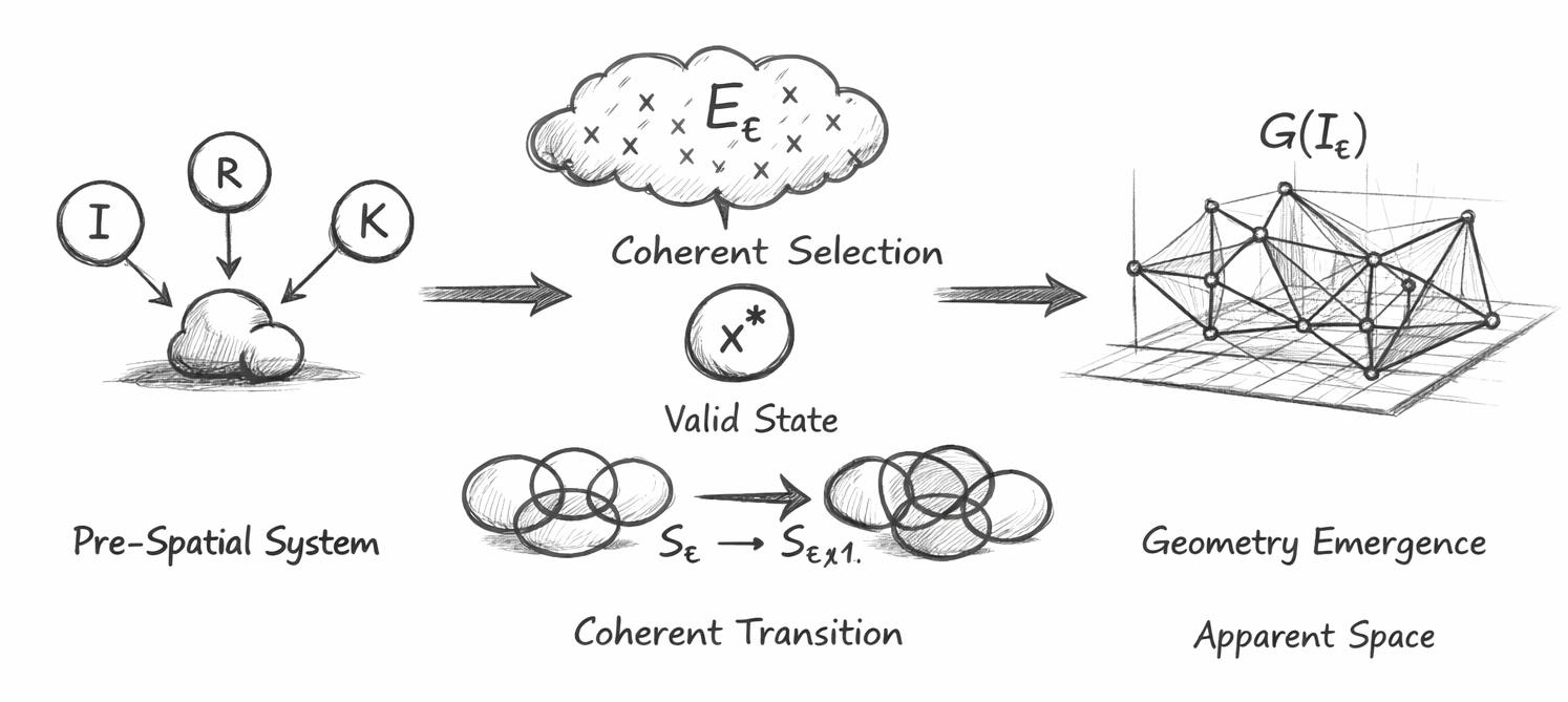
Pre-Spatial → Coherence → Geometry Emergence

1. Overview of the Diagram

The diagram represents a three-stage transformation pipeline:

Pre-Spatial System→Coherent Selection→Geometry Emergence

It visualises the central claim of Chapter 5:

Space is not fundamental—it emerges only after coherent continuation has been resolved.

Each region of the diagram corresponds directly to a stage in the Flow Algebra execution pipeline.

2. Left Region — Pre-Spatial System (Substrate Definition)

Visual Elements:
  • Nodes labelled II, RR, and KK converging into an undefined structure
  • No grid, coordinates, or geometric embedding
  • A “cloud-like” form representing unstructured relational content
Formal Correspondence:

\[ S = (I, R, B, K), \quad H = \varnothing \]


Scientific Interpretation:

This region depicts the pre-spatial substrate, where:

  • II encodes relational information
  • RR defines transformation rules
  • BB and KK impose constraints and invariants

Crucially:

  • There is no notion of position or distance
  • No spatial manifold exists
  • No geometry is assumed or implied

This enforces the principle:

\[ S \notin \{ I, R, B, K \} \]

Thus, the system is ontologically closed and pre-geometric.

3. Central Region — Expansion and Coherent Selection

3.1 Expansion Layer
Visual Elements:
  • A cloud labelled EtE_t containing multiple candidate points (× symbols)
  • Represents a branching of possible continuations
Formal Correspondence:

\[ E_t = \operatorname{expand}(I_t, R) \]

Interpretation:
  • All possible next states are generated
  • These are purely relational possibilities, not spatial configurations
3.2 Validation and Selection
Visual Elements:
  • A filtered subset collapsing to a single node x∗x^*
  • Labelled “Coherent Selection” and “Valid State”
Formal Correspondence:

\[ V_t = \{ x \in E_t \mid x \vDash (B \wedge K) \} \]

\[ x^* \in V_t \]

Scientific Interpretation:

This stage implements:

  • Constraint filtering (via BB, KK)
  • Resolution of coherence (selection of x∗x^*)

Key properties:

  • No spatial criteria are applied
  • Validity is purely logical and structural
  • The system selects a continuation based on coherence, not location
3.3 State Transition
Visual Elements:
  • Transition arrow: 𝑆 𝑡 → 𝑆 𝑡 + 1
  • Overlapping cluster forms indicating continuity
Formal Correspondence:

\[ I_{t+1} = \operatorname{update}(I_t, x^*) \]

Interpretation:
  • The system transitions to a new valid state
  • This is not motion through space, but replacement of state under constraint

4. Right Region — Geometry Emergence (Derived Structure)

Visual Elements:
  • A structured network overlaid on a grid
  • Nodes and edges forming a geometric pattern
  • Label: G(It)G(I_t)
Formal Correspondence:

\[ D_t = G(I_t) \]

Scientific Interpretation:

This region shows the emergence of apparent spatial structure:

  • Geometry arises from stable relational ordering
  • The grid is illustrative, not fundamental
  • Spatial properties are inferred, not assumed

Thus:

  • Distance = relational difference
  • Topology = constraint connectivity
  • Geometry = projection of coherence

5. Directionality and Causality

The diagram enforces a strict directional flow:

\[ (I, R, B, K) \rightarrow E_t \rightarrow V_t \rightarrow x^* \rightarrow I_{t+1} \rightarrow G(I_t) \]

Critically:

\[ G(I_t) \not\Rightarrow E_t,\quad G(I_t) \not\Rightarrow V_t,\quad G(I_t) \not\Rightarrow x^* \]

This ensures:

  • Geometry is non-causal
  • No circular dependency exists
  • Space cannot generate or validate itself

6. Key Scientific Insight Encoded

The diagram encodes the following structural hierarchy:

Coherence→Valid Continuation→Relational Stability→Geometry

NOT:

Space→Physics

7. Failure Condition (Implicit in Diagram)

Although not visually dominant, the diagram implies:

\[ V_t = \varnothing \;\Rightarrow\; \text{No } x^* \;\Rightarrow\; \text{No } I_{t+1} \;\Rightarrow\; \text{No } G(I) \]

Thus:

If coherence fails, geometry never emerges.

8. Interpretation for Physicists

To correctly read the diagram:
  • Treat the left and central regions as fundamental
  • Treat the right region as derived
  • Do not interpret arrows as spatial motion
  • Interpret all transitions as state evolution under constraint

9. Final Statement

The diagram formalises a complete inversion of classical ontology:

Space is not the stage of physics—it is the projection of successful coherence.

Diagram → Flow Mapping

The Myth of Spatial Primacy
Diagram Element Flow Algebra Equation Meaning
Left cluster (I, R, K nodes) System Definition \(S = (I, R, B, K),\; H = \varnothing\) Pre-spatial substrate (no geometry present)
Unstructured cloud (left) Initial State \(I_t\) Pure relational information (no coordinates)
Expansion cloud (Eₜ with ×) Expand \(E_t = \text{expand}(I_t, R)\) All possible next states generated
Filtered region → single node Validate + Select \(V_t = \{x \in E_t \mid x \models (B \wedge K)\},\; x^* \in V_t\) Coherent candidate selected
“Valid State” node (x*) Selection Output \(x^*\) Resolved continuation (not spatial motion)
Arrow Sₜ → Sₜ₊₁ Update \(I_{t+1} = \text{update}(I_t, x^*)\) State transition under constraints
Overlapping clusters Continuation \(S_t \rightarrow S_{t+1}\) Coherent evolution (no spatial traversal)
Right-hand geometric network Derived Structure \(D_t = G(I_t)\) Apparent geometry emerges from structure
Grid under network Interpretation Layer \(G(I)\) Visual encoding of relational coherence

How to Use This Table (Scientifically)

  • Read left → right as execution order
  • Treat:
  • Left + centre = fundamental process
  • Right = derived interpretation
  • Use the table to:
  • Anchor each visual element to a formal equation
  • Prevent misreading geometry as causal

Key Structural Insight

Diagram Flow≡Execution Pipeline

\[ (I, R, B, K) \rightarrow E_t \rightarrow V_t \rightarrow x^* \rightarrow I_{t+1} \rightarrow G(I_t) \]

Closing Note

This mapping ensures the diagram is not just illustrative—but formally exact.

Every visual element corresponds to a defined operation, and every operation preserves the core principle:

Geometry is the final layer—not the starting point.

Related Chapters
Kireth Research
38 Thorndale Croft, Wetwang, Driffield
East Riding of Yorkshire YO25 9XZ
Telephone: 01377 236594
Designed By