Chapter 37
Divergence as Coherence Flux

Maxwell Reformulated
Author: Mark Higgins
© Mark Anthony Higgins 11 October 2025
Revised Date: 11 June 2026
Audio Overview

Scientific Introduction

Divergence is one of the most fundamental operators in field theory, yet it is often introduced as a purely mathematical tool rather than a physical process. In conventional electromagnetism, fluid mechanics, gravitation, and continuum physics, divergence measures the net outward flow of a quantity from a region of space. Positive divergence indicates a source, negative divergence indicates a sink, and zero divergence implies conservation within the local volume.

While mathematically successful, the traditional interpretation leaves open a deeper question:

Telephone:
01377 236594
Why do sources and sinks exist at all?

Within the Holographic Space-Time (HST) framework, divergence is not merely a property of a vector field. Instead, it emerges from the movement of coherence through structured curvature geometry. A field does not possess divergence independently; rather, divergence appears whenever coherence enters or leaves a local boundary region.

This chapter reformulates divergence as a measurable manifestation of coherence flux.

Under HST, every physical field originates from coherence distributions encoded across boundaries. These coherence structures generate gradients, gradients generate tension, and tension produces curvature dynamics. As coherence moves through a region, local boundary geometry records whether coherence is accumulating, dispersing, or remaining balanced.

Divergence therefore becomes a direct measurement of local coherence flow.

37.1 The Classical View of Divergence

In standard vector calculus, divergence is defined as the scalar operator:

\[ \nabla \cdot F \]

where F represents a vector field.

The operator measures the net outward flux through an infinitesimal volume.

If:

  • Divergence > 0 → net outward flow
  • Divergence < 0 → net inward flow
  • Divergence = 0 → balanced flow

Examples include:

Electrostatics

Gauss's Law states that electric charge acts as a source of electric field divergence.

Fluid Dynamics

Divergence indicates whether fluid density increases or decreases locally.

Gravitation

Mass concentrations create convergence of field lines.

Electromagnetism

Electric fields may possess divergence while magnetic fields remain divergence-free.

Although these descriptions quantify field behaviour, they do not explain the underlying mechanism that produces sources and sinks.

37.2 The HST Perspective

HST begins from a different assumption.

Fields are not fundamental entities.

Instead:

  • 1. Boundaries encode coherence.
  • 2. Coherence distributions generate gradients.
  • 3. Gradients generate tension.
  • 4. Tension generates curvature.
  • 5. Curvature generates observable fields.

Under this framework, divergence measures the net rate at which coherence crosses a local boundary.

Rather than asking:

"How much field exits this volume?"

HST asks:

"How much coherence is entering or leaving the local geometric structure?"

The physical meaning shifts from field flow to coherence transport.

37.3 Coherence Flux

Consider a coherence density field:

\[ C(x,y,z,t) \]

representing the local organisation of information across the boundary structure.

As coherence moves through space, a coherence flow field develops:

\[ J_C \]

where:

  • JCJ_C = coherence current
  • direction = coherence transport direction
  • magnitude = coherence transport rate

The divergence of this current becomes:

\[ \nabla \cdot J_C \]

which measures the local imbalance of coherence transport.

Positive values indicate coherence emission.

Negative values indicate coherence accumulation.

Zero indicates dynamic equilibrium.

This quantity forms the HST interpretation of divergence.

37.4 Sources as Coherence Emission Regions

In conventional physics, a source is often treated as a primitive object.

Charge generates electric fields.

Mass generates gravitational fields.

Current generates magnetic fields.

HST instead interprets sources as regions where coherence is exported into surrounding geometry.

The local boundary possesses excess coherence density relative to its environment.

This imbalance drives outward coherence transport.

Consequently:

  • coherence leaves the region,
  • gradients form,
  • curvature develops,
  • field structures emerge.

Positive divergence therefore corresponds to coherence release.

The source is not generating fields directly.

The source is generating coherence flux.

37.5 Sinks as Coherence Absorption Regions

The opposite process creates negative divergence.

Here surrounding coherence converges toward a region of lower coherence potential.

The local structure absorbs coherence from neighbouring regions.

Observable consequences include:

  • field convergence,
  • gradient collapse,
  • curvature concentration,
  • energy localisation.

Negative divergence therefore corresponds to coherence absorption.

The sink is a coherence attractor.

37.6 Divergence-Free Fields

One of the most important concepts in physics is the existence of divergence-free fields.

The classic example is magnetism:

\[ \nabla \cdot \mathbf{B} = 0 \]

meaning magnetic field lines possess no beginning and no end.

Within HST this becomes a coherence conservation statement.

Magnetic structures correspond to closed coherence circulation loops.

Coherence continuously redistributes through the loop without net creation or destruction.

Therefore:

  • no local emission exists,
  • no local absorption exists,
  • total coherence remains balanced.

Divergence-free behaviour emerges naturally from closed coherence topology.

37.7 Geometric Interpretation

A useful geometric picture is to imagine every point in space surrounded by a microscopic coherence boundary.

The boundary behaves like a flexible membrane.

If coherence exits faster than it enters:

  • the membrane expands outward,
  • positive divergence appears.

If inflow equals outflow:

  • geometry remains stable,
  • divergence vanishes

Thus divergence measures how local boundary geometry responds to coherence transport.

37.8 Relationship to Gauss's Law

Gauss's Law traditionally states that the total electric flux through a closed surface equals the enclosed charge.

HST reformulates this as:

Total coherence flux through a closed boundary equals the enclosed coherence displacement.

Charge becomes a geometric manifestation of coherence imbalance.

Electric field divergence becomes a measurement of coherence emission from displaced curvature structures.

The classical law remains mathematically unchanged.

Only the physical interpretation changes.

37.9 Divergence and Conservation

The conservation laws of physics become especially transparent within this framework.

If coherence cannot be created or destroyed globally, then positive divergence in one region must ultimately be balanced by negative divergence elsewhere.

Local divergence may exist.

Global divergence must sum to zero.

Thus conservation laws emerge naturally from coherence accounting across the complete boundary network.

This interpretation links:

  • charge conservation,
  • energy conservation,
  • information conservation,
  • field continuity,

into a single coherence-flux framework.

37.10 Chapter Summary

Divergence is traditionally viewed as the net outward flow of a vector field from a region of space.

Within HST, divergence acquires a deeper physical interpretation.

It becomes a direct measure of coherence flux across local boundary structures.

Under this reformulation:

  • Positive divergence corresponds to coherence emission.
  • Negative divergence corresponds to coherence absorption.
  • Zero divergence corresponds to coherence equilibrium.
  • Sources become coherence exporters.
  • Sinks become coherence attractors.
  • Divergence-free fields become closed coherence circulation systems.

The mathematical operator remains unchanged.

What changes is its meaning.

Divergence is no longer merely a property of a field.

It becomes a measurable signature of how coherence moves through the geometric fabric from which fields themselves emerge.

flow "Divergence_as_Coherence_Flux" v1.0

PURPOSE:
Reformulate divergence as the local measurement of coherence flux through a bounded region.
In HST, divergence does not describe field flow alone; it describes whether coherence is
leaving, entering, or balancing across a local boundary structure.

AUTHORS:
- Mark Higgins
- Sky

DOMAIN:
Holographic Space-Time theory
Electromagnetism
Field geometry
Boundary coherence physics

INPUTS:
  It:
    description: Local boundary-encoded information state.
    type: boundary_information_state

  Bt:
    description: Local boundary region enclosing the field sample volume.
    type: bounded_coherence_surface

  Ct:
    description: Coherence density distribution over the boundary region.
    type: scalar_coherence_field

  Jc_t:
    description: Coherence current through the local boundary.
    type: vector_coherence_flux_field

  Ft:
    description: Observable field produced from coherence transport.
    type: emergent_vector_field

STATE_VARIABLES:
  Ct:
    meaning: Local coherence density.
    expression: C(x,y,z,t)

  Jc_t:
    meaning: Coherence current.
    expression: J_C(x,y,z,t)

  DivC_t:
    meaning: Local coherence divergence.
    expression: ∇ · J_C

  PhiC_t:
    meaning: Total coherence flux through closed boundary.
    expression: ∮ J_C · dA

  Qt:
    meaning: Enclosed coherence displacement.
    expression: Q_C = ∫ DivC_t dV

  St:
    meaning: Current physical-coherence state.
    expression: S_t = (I_t, B_t, C_t, J_C,t)

  St_plus_1:
    meaning: Updated physical-coherence state.
    expression: S_{t+1}

PROCESS:
  R1_Map_Boundary_Coherence:
    input: It
    operation: Extract coherence structure from local boundary information.
    output: Ct
    rule: It -> Ct

  R2_Form_Coherence_Gradient:
    input: Ct
    operation: Detect spatial variation in coherence density.
    output: GradC_t
    rule: Ct -> ∇Ct

  R3_Generate_Coherence_Current:
    input: ∇Ct
    operation: Coherence moves along local imbalance paths.
    output: Jc_t
    rule: J_C,t = flow(∇Ct)

  R4_Measure_Local_Divergence:
    input: Jc_t
    operation: Measure net coherence leaving or entering a local volume.
    output: DivC_t
    rule: DivC_t = ∇ · J_C,t

  R5_Classify_Coherence_Flux:
    input: DivC_t
    operation: Determine whether the region is a source, sink, or balanced structure.
    output: FluxState_t
    rules:
      if DivC_t > 0:
        FluxState_t = COHERENCE_SOURCE
      if DivC_t < 0:
        FluxState_t = COHERENCE_SINK
      if DivC_t = 0:
        FluxState_t = COHERENCE_BALANCE

  R6_Integrate_Closed_Surface_Flux:
    input: Jc_t, Bt
    operation: Sum coherence flux through the closed boundary surface.
    output: PhiC_t
    rule: PhiC_t = ∮_Bt J_C,t · dA

  R7_Map_Flux_To_Enclosed_Displacement:
    input: DivC_t
    operation: Convert local divergence into enclosed coherence displacement.
    output: Qt
    rule: Q_C = ∫_V DivC_t dV

  R8_Generate_Observable_Field:
    input: Qt, GradC_t, Jc_t
    operation: Produce observable field behaviour from coherence displacement and flux.
    output: Ft
    rule: Ft = field(Q_C, ∇Ct, J_C,t)

  R9_Update_State:
    input: St, Ft, FluxState_t
    operation: Update the physical-coherence state after coherence transport.
    output: St_plus_1
    rule: S_t -> S_{t+1}

INVARIANTS:
  I1_Global_Coherence_Conservation:
    statement: Total coherence cannot be created or destroyed globally.
    expression: ∫_AllSpace DivC_t dV = 0

  I2_Local_Source_Sink_Balance:
    statement: Positive local divergence must be balanced by negative divergence elsewhere.
    expression: Σ DivC_positive + Σ DivC_negative = 0

  I3_Divergence_Free_Closed_Loops:
    statement: Closed coherence circulation has no local source or sink.
    expression: ∇ · J_C = 0

  I4_Boundary_Flux_Consistency:
    statement: Surface flux must equal enclosed coherence displacement.
    expression: ∮_Bt J_C · dA = ∫_V ∇ · J_C dV

  I5_Field_Emergence_Consistency:
    statement: Observable field divergence must correspond to coherence flux imbalance.
    expression: ∇ · F_t ∝ ∇ · J_C,t

CONDITIONS:
  SOURCE_STATE:
    when: ∇ · J_C,t > 0
    meaning: Coherence exits the region faster than it enters.
    interpretation: Local region behaves as a field source.

  SINK_STATE:
    when: ∇ · J_C,t < 0
    meaning: Coherence enters the region faster than it exits.
    interpretation: Local region behaves as a field sink.

  BALANCED_STATE:
    when: ∇ · J_C,t = 0
    meaning: Coherence inflow equals coherence outflow.
    interpretation: Local field remains divergence-free.

  FAILURE_STATE:
    when: global conservation is violated
    meaning: Coherence accounting is inconsistent.
    output: EXECUTION_FAIL

OUTPUTS:
  DivC_t:
    description: Local coherence divergence.
    expression: ∇ · J_C,t

  PhiC_t:
    description: Total coherence flux through the closed boundary.
    expression: ∮ J_C,t · dA

  Qt:
    description: Enclosed coherence displacement.
    expression: Q_C

  FluxState_t:
    description: Source, sink, or balanced coherence classification.

  Ft:
    description: Emergent observable field.

  St_plus_1:
    description: Updated coherence-field state.

EXECUTION_CHAIN:
  It -> Ct -> ∇Ct -> J_C,t -> ∇ · J_C,t -> FluxState_t -> PhiC_t -> Q_C -> Ft -> S_{t+1}

SCIENTIFIC_INTERPRETATION:
  Divergence is the local scalar measurement of coherence flux.
  Positive divergence means coherence emission.
  Negative divergence means coherence absorption.
  Zero divergence means closed or balanced coherence circulation.
  Classical field divergence is preserved mathematically but reinterpreted as boundary-coherence transport.

EXECUTION_GUARANTEE:
  If coherence flux is locally measurable and globally conserved, divergence is validly interpreted
  as coherence transport across boundary geometry. If local divergence cannot be balanced globally,
  the system fails coherence conservation and cannot produce a stable physical field state.

What This Flow Implements

Overview

This flow implements a complete Holographic Space-Time (HST) reformulation of divergence by replacing the traditional interpretation of divergence as merely a mathematical property of a vector field with a physical interpretation based on coherence transport.

In conventional physics, divergence measures the net outward flow of a vector quantity through an infinitesimal volume. While mathematically precise, the operator itself provides little insight into why sources, sinks, and divergence-free structures emerge in nature.

The purpose of this flow is to provide a deeper physical mechanism.

Within HST, divergence is interpreted as the measurable signature of coherence moving through local boundary geometry. Observable field divergence becomes a secondary effect of a more fundamental process: the transport of coherence across structured boundaries.

The flow therefore implements a causal chain linking information structure, coherence density, coherence current, divergence generation, flux classification, and emergent field behaviour.

Fundamental Principle Implemented

The core principle implemented by this flow is:

Divergence is not fundamentally a property of a field. Divergence is the local measurement of coherence flux through boundary geometry.

The flow assumes that physical fields emerge from coherence distributions encoded across boundaries.

Under this interpretation:

Information→Coherence→Gradient→
Flux→Divergence→Field

rather than:

Source→Field→Divergence

This reversal of causality is one of the central HST reinterpretations implemented by the flow.

Boundary-to-Divergence Transformation

The first stage of the flow implements the conversion of information structures into coherence structures.

The system begins with:

\[ I_t \]

representing the informational state of a local boundary.

The flow maps this information into a coherence distribution:

representing the informational state of a local boundary.

The flow maps this information into a coherence distribution:

\[ I_t \rightarrow C_t \]

This operation represents the HST assumption that all observable physical behaviour originates from organised coherence patterns embedded within boundary geometry.

At this stage no fields yet exist.

Only coherence organisation exists.

Coherence Gradient Formation

The second stage implements gradient generation.

Spatial variations in coherence density produce:

\[ \nabla C_t \]

which represents the local direction of coherence imbalance.

The gradient identifies where coherence density is increasing or decreasing across the surrounding geometry.

This stage establishes the directional structure required for transport.

Without gradients there is no preferred direction of motion and therefore no divergence.

Coherence Current Generation

Once gradients exist, the flow implements coherence transport.

This creates the coherence current:

\[ J_C \]

which acts as the fundamental transport quantity within the model.

The coherence current represents:

  • direction of coherence movement,
  • magnitude of coherence transfer,
  • local transport rate.

This is the first stage where dynamic behaviour appears.

The flow therefore transforms a static coherence landscape into an active coherence transport system.

Divergence Generation

The central operation implemented by the flow is:

\[ \nabla \cdot J_C \]

This computes the local balance between coherence entering and leaving a bounded region.

The divergence operator is reinterpreted as a coherence accounting mechanism.

Instead of measuring field expansion directly, the operator measures whether coherence is accumulating, dispersing, or remaining balanced.

This stage forms the heart of the HST divergence model.

Source Detection

The flow implements automatic identification of coherence sources.

When:

\[ \nabla \cdot J_C > 0 \]

the system classifies the region as a coherence emitter.

This indicates that coherence leaves the local volume faster than it enters.

Within HST this corresponds to:

  • outward coherence transport,
  • curvature release,
  • field generation,
  • source-like behaviour.

Classical electric charge becomes one example of this process.

The flow therefore reinterprets physical sources as regions of net coherence emission.

Sink Detection

The flow also implements identification of coherence sinks.

When:

\[ \nabla \cdot J_C < 0 \]

the region becomes a coherence absorber.

This indicates:

  • inward coherence transport,
  • coherence accumulation,
  • gradient convergence,
  • sink-like behaviour.

The flow therefore provides a physical mechanism for field convergence.

Rather than treating sinks as mathematical abstractions, the system interprets them as coherence attractors embedded within boundary geometry.

Divergence-Free Structures

A major feature implemented by the flow is recognition of divergence-free coherence systems.

When:

\[ \nabla \cdot J_C = 0 \]

the coherence current forms a balanced transport network.

This condition corresponds to:

  • closed coherence circulation,
  • equilibrium transport,
  • conserved local coherence,
  • stable field loops.

The most important example is magnetism:

\[ \nabla \cdot \mathbf{B} = 0 \]

Within HST, the flow interprets this condition as evidence of closed coherence circulation rather than the absence of field structure.

The field remains active while coherence remains globally balanced.

Closed Boundary Flux Implementation

The flow implements the full boundary-flux relationship.

Total coherence flux through a closed boundary is computed as:

\[ \Phi_C = \oint J_C \cdot dA \]

This operation measures total coherence crossing the boundary surface.

The flow therefore captures both:

  • local divergence behaviour,
  • global boundary behaviour.

This creates a direct HST analogue of Gauss-type conservation relationships.

Enclosed Coherence Displacement

The flow integrates divergence throughout a volume to calculate:

\[ Q_C = \int_V \left( \nabla \cdot J_C \right) \, dV \]

which represents enclosed coherence displacement.

This quantity acts as the HST equivalent of enclosed source strength.

The implementation therefore connects:

Local Divergence

↓

Boundary Flux

↓

Enclosed Coherence Displacement

↓

Observable Field Behaviour

into a single continuous causal chain.

Emergent Field Construction

The flow implements field emergence as a consequence of coherence transport.

Observable fields are generated from:

  • coherence gradients,
  • coherence currents,
  • coherence displacement.

Thus:

\[ F_t = \mathrm{field} \!\left( Q_C,\, \nabla C_t,\, J_C \right) \]

This replaces the traditional assumption that fields are primary entities.

The flow instead treats fields as observable manifestations of deeper coherence dynamics.

Conservation Enforcement

A critical implementation within the flow is global coherence conservation.

The invariant:

\[ \int_{\mathrm{All\ Space}} \left( \nabla \cdot J_C \right) \, dV = 0 \]

ensures that total coherence remains conserved across the entire system.

This means:

  • local sources may exist,
  • local sinks may exist,
  • global coherence creation is forbidden,
  • global coherence destruction is forbidden.

The flow therefore embeds conservation directly into its execution rules.

Relationship to Classical Physics

This flow preserves every mathematical operation used in conventional divergence theory.

The divergence operator remains unchanged.

The surface integral remains unchanged.

The conservation relationships remain unchanged.

What changes is the interpretation.

Traditional Physics:

Field→Divergence

HST:

Coherence→Flux→Divergence→Field

Thus the flow provides a deeper explanatory layer while remaining mathematically compatible with established field theory.

Scientific Significance

This flow implements one of the most important conceptual transitions within HST field physics.

It transforms divergence from a purely mathematical operator into a physically interpretable measure of coherence transport.

By doing so, the flow provides a unified explanation for:

  • field sources,
  • field sinks,
  • divergence-free systems,
  • Gauss-type conservation laws,
  • charge-like behaviour,
  • flux conservation,
  • boundary-driven field emergence.

The result is a framework in which divergence becomes a direct observational signature of coherence moving through the geometric structure from which physical fields arise.

How to Read This Flow

Introduction

At first glance, the Divergence as Coherence Flux flow may appear similar to a conventional field-theory model because it contains familiar concepts such as gradients, flux, divergence, sources, sinks, and conservation laws. However, the purpose of this flow is fundamentally different.

Traditional physics typically begins with fields and then calculates divergence as a mathematical property of those fields.

This flow reverses that relationship.

The flow begins with information encoded on boundaries and demonstrates how coherence transport naturally produces divergence, which subsequently manifests as observable field behaviour.

To read the flow correctly, think of it as a causal chain that explains the origin of divergence rather than merely calculating it.

Reading Philosophy

The flow should be read from left to right:

Information
    ↓
Coherence
    ↓
Gradient
    ↓
Flux
    ↓
Divergence
    ↓
Field

Each stage produces the next stage.

Nothing appears spontaneously.

Every observable effect must arise from a prior coherence process.

This causal structure is central to the HST interpretation.

Step 1 — Information State

The flow begins with:

It

which represents the informational structure encoded within a local boundary region.

This is the deepest layer of the model.

The information state contains the organisation that later becomes coherence.

When reading the flow:

It → Ct

interpret this as:

Information is converted into a measurable coherence distribution.

At this stage:

  • no field exists,
  • no divergence exists,
  • no flux exists.

Only structured information is present.

Step 2 — Coherence Distribution

The next state is:

Ct

representing coherence density throughout the local region.

The flow assumes that information organises into coherence patterns.

These patterns determine:

  • stability,
  • structure,
  • potential transport directions.

When reading:

Ct

imagine a three-dimensional coherence landscape.

Some regions contain higher coherence density.

Other regions contain lower coherence density.

These differences become important in the next stage.

Step 3 — Coherence Gradient Formation

The flow then generates:

∇Ct

which represents the spatial variation of coherence.

This is the first location where direction appears.

A gradient identifies:

  • where coherence is concentrated,
  • where coherence is depleted,
  • where imbalance exists.

Read:

Ct → ∇Ct

as:

Coherence imbalance creates directional potential.

Without gradients:

∇Ct = 0

there can be:

  • no preferred direction,
  • no transport,
  • no divergence.

The system remains static.

Step 4 — Coherence Current Generation

The next operation is:

JC,t = flow(∇Ct)

This creates the coherence current:

JC,t

which describes how coherence moves through space.

This is analogous to:

  • electric current,
  • fluid flow,
  • heat transport,

but applied to coherence itself.

When reading this stage imagine coherence physically moving through the local geometry.

The flow has now become dynamic.

Telephone:
01377 236594

Step 5 — Local Divergence Measurement

This is the central operation of the entire chapter:

DivC,t = ∇ · JC,t

The divergence operator measures whether coherence is leaving or entering a local volume.

Read this stage as:

Measure the net balance of coherence transport.

This operation determines whether the region behaves as:

  • a source,
  • a sink,
  • a balanced structure.

The result is:

DivC,t

which is the local coherence divergence.

Step 6 — Source Interpretation

The flow contains the condition:

∇ · JC,t > 0

When reading this condition:

interpret it as:

More coherence leaves the region than enters it.

The region behaves as a coherence source.

In physical terms:

  • coherence is emitted,
  • gradients expand,
  • fields emerge outward.

The flow labels this state:

COHERENCE_SOURCE

This corresponds to positive divergence.

Step 7 — Sink Interpretation

The second classification is:

∇ · JC,t < 0

Read this as:

More coherence enters the region than leaves it.

The region becomes a coherence sink.

Consequences include:

  • inward transport,
  • convergence,
  • accumulation.

The flow labels this state:

COHERENCE_SINK

This corresponds to negative divergence.

Step 8 — Balanced Coherence State

The third possibility is:

∇ · JC,t = 0

Read this as:

Coherence entering equals coherence leaving.

No net accumulation occurs.

No net emission occurs.

The region becomes:

COHERENCE_BALANCE

This is one of the most important states in field theory because it corresponds to divergence-free systems.

Examples include closed circulation structures such as magnetic field loops.

Step 9 — Boundary Flux Integration

The next section computes total coherence flux through a closed surface:

PhiC,t = ∮ JC,t · dA

Read this operation as:

Measure all coherence crossing the boundary.

Unlike local divergence, which measures behaviour at a point, this operation measures behaviour across an entire enclosed surface.

This provides the global view of coherence transport.

Step 10 — Enclosed Coherence Displacement

The flow then computes:

QC = ∫V DivC,t dV

This determines the total coherence displacement enclosed within the volume.

Read this as:

Calculate the total coherence imbalance contained inside the boundary.

This stage links local divergence measurements to large-scale field behaviour.

Step 11 — Field Emergence

The flow generates the observable field through:

Ft = field(QC, ∇Ct, JC,t)

This is the point where physical fields appear.

Read this carefully.

The field is not the starting point.

The field is the result.

The flow therefore follows:

Coherence
    ↓
Flux
    ↓
Divergence
    ↓
Field

rather than:

Field
    ↓
Divergence

This distinction is one of the key HST concepts implemented by the flow.

Step 12 — State Update

The final operation is:

St → St+1

which advances the system forward.

Read this as:

The coherence-field system evolves into its next physical state.

The process can then repeat recursively.

This allows divergence behaviour to evolve continuously through time.


Reading the Invariants

The invariants should be interpreted as rules that can never be violated during successful execution.

For example:

∫AllSpace DivC,t dV = 0

means:

Total coherence must remain globally conserved.

Likewise:

∮Bt JC · dA = ∫V ∇ · JC dV

states:

Boundary flux must equal enclosed coherence displacement.

These invariants guarantee that the flow remains physically self-consistent.

Reading the Execution Chain

The complete execution chain is:

It
→ Ct
→ ∇Ct
→ JC,t
→ ∇·JC,t
→ FluxStatet
→ PhiC,t
→ QC
→ Ft
→ St+1

Read this chain as a complete causal narrative:

Information creates coherence.

Coherence creates gradients.

Gradients create transport.

Transport creates divergence.

Divergence creates sources and sinks.

Sources and sinks create field behaviour.

Field behaviour updates reality.

This single sequence encapsulates the entire purpose of the flow.

Scientific Interpretation

The flow is not intended merely to calculate divergence.

It is intended to explain divergence.

Every section should therefore be read as part of a deeper physical story:

Boundary Information
        ↓
Coherence Organisation
        ↓
Coherence Motion
        ↓
Coherence Flux
        ↓
Divergence
        ↓
Field Emergence

Under this interpretation, divergence becomes a measurable signature of coherence transport through boundary geometry, providing the physical mechanism from which sources, sinks, and divergence-free field structures naturally emerge.

Flow → Equation Tri-Mapping Table

Flow Layer Flow Algebra Expression HST Equation Layer Classical Physics Equivalent Scientific Interpretation
Information State I_t I_t Initial system state Boundary-encoded information structure
Boundary Mapping I_t → C_t C_t = CoherenceMap(I_t) Field initialization Information organised into coherence density
Coherence Density C_t C(x,y,z,t) Scalar potential distribution Spatial coherence landscape
Gradient Formation C_t → ∇C_t ∇C_t Potential gradient Direction of coherence imbalance
Gradient Field ∇C_t ∂C/∂x, ∂C/∂y, ∂C/∂z Electric potential gradient Local coherence variation
Flux Generation ∇C_t → J_C,t J_C,t = f(∇C_t) Current density (J) Coherence transport current
Coherence Current J_C,t J_C(x,y,z,t) Flux vector field Direction and magnitude of coherence flow
Divergence Operator J_C,t → DivC_t DivC_t = ∇·J_C,t ∇·F Net coherence flux density
Positive Divergence DivC_t > 0 ∇·J_C > 0 Source region Net coherence emission
Negative Divergence DivC_t < 0 ∇·J_C < 0 Sink region Net coherence absorption
Zero Divergence DivC_t = 0 ∇·J_C = 0 Divergence-free field Balanced coherence circulation
Source Classification FluxState_t = SOURCE ∇·J_C > 0 Positive charge density Local coherence exporter
Sink Classification FluxState_t = SINK ∇·J_C < 0 Negative charge density Local coherence attractor
Balanced Classification FluxState_t = BALANCE ∇·J_C = 0 Magnetic loop condition Closed coherence loop
Surface Flux Φ_C,t Φ_C,t = ∮ J_C · dA Gauss flux integral Total coherence crossing boundary
Volume Divergence Q_C Q_C = ∫V (∇·J_C) dV Enclosed source strength Total coherence displacement
Flux Conservation ∮J_C·dA = ∫V ∇·J_C dV Divergence Theorem Gauss Theorem Boundary flux equals internal divergence
Field Emergence Q_C,∇C_t,J_C → F_t F_t = field(Q_C,∇C_t,J_C) Electromagnetic field generation Observable field from coherence transport
Electric Field Mapping DivC_t → E_t ∇·E = ρ/ε₀ Gauss's Law Coherence displacement manifests as electric divergence
Magnetic Field Mapping DivC_t = 0 ∇·B = 0 Maxwell magnetic law Closed coherence circulation
Local Conservation DivC_source + DivC_sink = 0 Σ DivC = 0 Charge conservation Local source-sink balancing
Global Conservation I1 ∫AllSpace ∇·J_C dV = 0 Global conservation law Total coherence conserved
State Evolution S_t → S_t+1 S_t+1 = f(S_t) Field evolution equations Recursive coherence transport
Execution Chain I_t → C_t → ∇C_t → J_C → ∇·J_C → F_t Full HST Divergence Pipeline Field-theory evolution sequence Divergence emerges from coherence flux

Ultra-Tight Flow ⇄ Equation ⇄ Physics Summary

Flow HST Equation Physical Meaning
I_t I_t Boundary information
I_t → C_t C_t = CoherenceMap(I_t) Information becomes coherence
C_t C(x,y,z,t) Coherence density field
C_t → ∇C_t ∇C_t Coherence gradient
∇C_t → J_C J_C = f(∇C_t) Coherence transport
J_C → DivC_t ∇·J_C Coherence flux density
DivC_t > 0 ∇·J_C > 0 Source behaviour
DivC_t < 0 ∇·J_C < 0 Sink behaviour
DivC_t = 0 ∇·J_C = 0 Balanced circulation
Φ_C ∮ J_C · dA Total boundary flux
Q_C ∫V ∇·J_C dV Enclosed coherence displacement
F_t F_t = field(Q_C,∇C_t,J_C) Emergent physical field
S_t → S_t+1 S_t+1 = f(S_t) Recursive evolution

Core HST Identity

It→Ct→∇Ct→JC→∇⋅JC→Ft→St+1I_t \rightarrow C_t \rightarrow \nabla C_t \rightarrow J_C \rightarrow \nabla\cdot J_C \rightarrow F_t \rightarrow S_{t+1}

Interpretation: Information generates coherence, coherence generates gradients, gradients generate flux, flux generates divergence, divergence generates observable fields, and fields update the next physical state. This is the complete HST reformulation of divergence as coherence flux.

Chapter 37 — Divergence as Coherence Flux

Overview

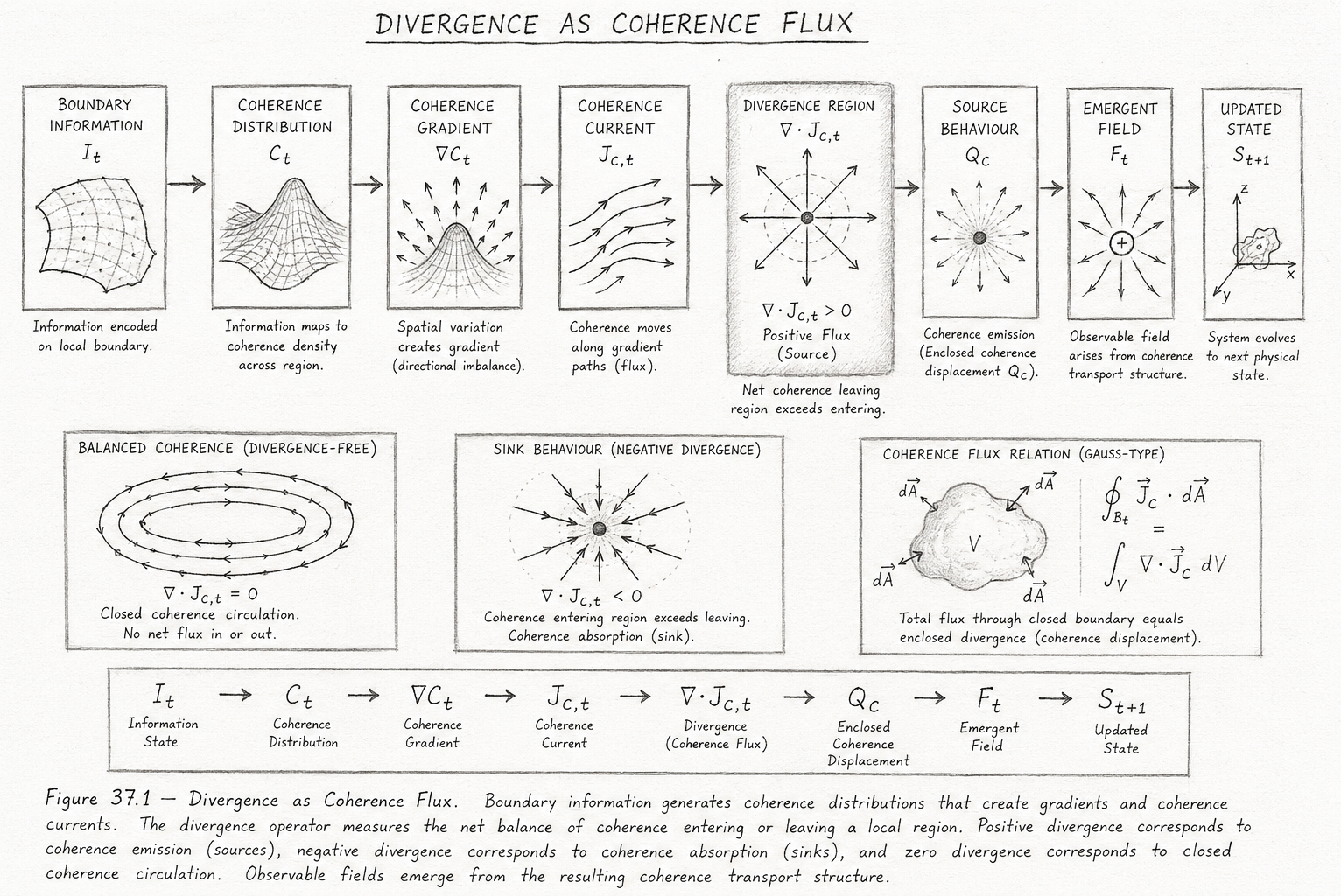
Figure 37.1 illustrates the Holographic Space-Time (HST) interpretation of divergence as a manifestation of coherence transport through boundary geometry. Rather than treating divergence as a purely mathematical operator applied to an existing field, the diagram presents divergence as the measurable result of coherence moving through structured space.

The figure traces the complete causal chain from boundary information to emergent field behaviour, showing how local coherence imbalances generate gradients, gradients generate transport currents, and transport currents produce divergence. Observable fields arise as a consequence of these deeper coherence processes.

The diagram therefore provides a physical interpretation for the divergence operator while preserving its mathematical form.

Boundary Information Layer

The first panel represents the informational state of the boundary:

\[ I_t \]

Within HST, physical reality begins as structured information encoded across boundaries.

The irregular mesh illustrates that the boundary is not an empty geometric surface but an information-bearing structure capable of storing coherence relationships.

At this stage:

  • no field exists,
  • no flux exists,
  • no divergence exists.

Only informational organisation is present.

The diagram therefore begins at the deepest layer of the HST hierarchy.

Coherence Distribution Layer

The second panel shows the emergence of a coherence density field:

\[ C_t \]

The curved surface represents the spatial distribution of coherence throughout the local region.

Higher elevations correspond to regions of greater coherence density.

Lower elevations correspond to reduced coherence density.

This panel illustrates the transition:

\[ I_t \rightarrow C_t \]

meaning that boundary information becomes physically represented as coherence organisation.

The coherence field forms the substrate from which all subsequent dynamics emerge.

Coherence Gradient Layer

The third panel introduces:

\[ \nabla C_t \]

the coherence gradient.

The arrows indicate the direction of greatest coherence variation.

This is the first point in the diagram where directional behaviour appears.

The gradient identifies:

  • coherence excess,
  • coherence deficit,
  • transport direction.

Physically, the gradient represents stored geometric imbalance.

Without gradients there would be no preferred direction for coherence movement and therefore no mechanism for divergence generation.

Coherence Current Layer

The fourth panel introduces the coherence current:

\[ J_C \]

The flowing arrows represent coherence moving through the local geometric structure.

This stage transforms a static coherence landscape into a dynamic transport system.

The coherence current serves the same structural role that electric current serves in electromagnetism or fluid velocity serves in hydrodynamics.

However, the transported quantity is coherence itself.

The panel represents the relationship:

\[ \nabla C_t \rightarrow J_C \]

showing that transport arises from coherence imbalance.

Divergence Region

The central panel is the most important component of the figure.

It depicts the divergence operator acting on the coherence current:

\[ \nabla \cdot J_C \]

The arrows radiating outward from the central point indicate that more coherence leaves the region than enters it.

This corresponds to:

\[ \nabla \cdot J_C > 0 \]

which the diagram labels as positive flux.

In the HST framework this does not merely describe field expansion.

Instead it indicates that coherence is being exported from the local boundary structure.

The panel therefore represents a coherence source.

Divergence becomes a direct measure of coherence emission.

Source Behaviour

The next panel expands the physical interpretation of positive divergence.

The outward-radiating coherence vectors illustrate coherence being released into surrounding geometry.

The enclosed coherence displacement:

\[ Q_C \]

represents the total coherence imbalance contained within the region.

This displacement acts as the underlying cause of observable source behaviour.

In conventional electromagnetism this role is played by electric charge.

Within HST the source is reinterpreted as a local coherence exporter.

Emergent Field Layer

The field panel demonstrates the appearance of an observable field:

\[ F_t \]

The central displacement generates a surrounding field structure represented by the radial arrows.

Importantly, the diagram places the field after divergence rather than before it.

This ordering reflects the HST causal sequence:

Coherence→Flux→Divergence→Field

rather than the conventional view in which divergence is merely computed from a pre-existing field.

The field therefore emerges from coherence transport dynamics

Updated State Layer

The final panel represents:

\[ S_{t+1} \]

the next physical state of the system.

The coordinate axes indicate that the coherence-field structure now exists as part of an updated geometric configuration.

This panel emphasises that the process is recursive.

Once a new state is produced, the entire sequence may repeat:

\[ S_t \rightarrow S_{t+1} \]

allowing divergence behaviour to evolve continuously through time.

Balanced Coherence Inset

The lower-left inset illustrates the special case:

\[ \nabla \cdot J_C = 0 \]

The closed circulating arrows represent a coherence loop in which inflow and outflow remain perfectly balanced.

No net coherence enters or leaves the region.

This corresponds to a divergence-free system.

The diagram visually demonstrates that zero divergence does not imply the absence of activity.

Coherence continues to circulate.

The circulation simply remains balanced.

This provides the HST interpretation of divergence-free field structures such as magnetic loops.

Sink Behaviour Inset

The lower-centre inset depicts:

\[ \nabla \cdot J_C < 0 \]

The inward-pointing arrows show coherence converging toward the centre.

This represents a coherence sink.

More coherence enters the region than leaves it.

The local geometry acts as a coherence attractor.

In HST this corresponds to coherence absorption, gradient collapse, and curvature concentration.

The inset therefore provides the counterpart to the positive-divergence source structure shown in the main diagram.

Coherence Flux Relation Inset

The lower-right inset presents the HST version of the divergence theorem.

The surface integral:

\[ \oint_{B_t} J_C \cdot dA \]

measures total coherence flux crossing the boundary.

The volume integral:

\[ \int_V \nabla \cdot J_C \, dV \]

measures total enclosed coherence displacement.

The equality between these quantities demonstrates that local coherence divergence and global boundary flux describe the same physical process viewed from different scales.

This inset forms the conservation bridge linking local coherence transport to large-scale field behaviour.

Bottom Execution Chain

The execution chain summarises the complete causal architecture:

\[ I_t \rightarrow C_t \rightarrow \nabla C_t \rightarrow J_C \rightarrow \nabla \cdot J_C \rightarrow Q_C \rightarrow F_t \rightarrow S_{t+1} \]

This sequence encapsulates the entire HST reformulation.

Information creates coherence.

Coherence creates gradients.

Gradients create transport.

Transport creates divergence.

Divergence creates field behaviour.

Field behaviour updates reality.

Telephone:
01377 236594

Scientific Significance

The significance of Figure 37.1 is that it transforms divergence from a mathematical descriptor into a physical mechanism.

Under this interpretation:

  • Positive divergence becomes coherence emission.
  • Negative divergence becomes coherence absorption.
  • Zero divergence becomes balanced coherence circulation.
  • Flux conservation becomes coherence conservation.
  • Sources become coherence exporters.
  • Sinks become coherence attractors.
  • Fields become observable manifestations of coherence transport.

The diagram therefore serves as a visual summary of the HST principle that divergence is fundamentally a measure of coherence flux moving through the geometric structure of reality.

Diagram → Flow Mapping Table

Flow HST Equation Physical Meaning
I_t I_t Boundary information
I_t → C_t C_t = CoherenceMap(I_t) Information becomes coherence
C_t C(x,y,z,t) Coherence density field
C_t → ∇C_t ∇C_t Coherence gradient
∇C_t → J_C J_C = f(∇C_t) Coherence transport
J_C → DivC_t ∇·J_C Coherence flux density
DivC_t > 0 ∇·J_C > 0 Source behaviour
DivC_t < 0 ∇·J_C < 0 Sink behaviour
DivC_t = 0 ∇·J_C = 0 Balanced circulation
Φ_C ∮ J_C · dA Total boundary flux
Q_C ∫V ∇·J_C dV Enclosed coherence displacement
F_t F_t = field(Q_C,∇C_t,J_C) Emergent physical field
S_t → S_t+1 S_t+1 = f(S_t) Recursive evolution

Ultra-Tight Diagram → Flow Summary

Diagram Region Flow Expression Meaning
Boundary Mesh I_t Boundary information
Coherence Surface C_t Coherence density
Gradient Arrows ∇C_t Coherence imbalance
Flow Streamlines J_C Coherence transport
Source Region ∇·J_C > 0 Coherence emission
Sink Region ∇·J_C < 0 Coherence absorption
Loop Region ∇·J_C = 0 Balanced circulation
Surface Integral ∮ J_C · dA Boundary flux
Volume Integral ∫V ∇·J_C dV Enclosed displacement
Field Region F_t Emergent field
Final State S_t+1 Updated reality

Complete Diagram Logic

𝐼 𝑡 → 𝐶 𝑡 → ∇ 𝐶 𝑡 → 𝐽 𝐶 → ∇ ⋅ 𝐽 𝐶 → 𝑄 𝐶 → 𝐹 𝑡 → 𝑆 𝑡 + 1 It​→Ct​→∇Ct​→JC​→∇⋅JC​→QC​→Ft​→St+1​

Diagram Interpretation: The figure visualises the complete HST divergence mechanism. Boundary information generates coherence organisation, coherence organisation generates gradients, gradients generate coherence currents, coherence currents generate divergence, divergence generates coherence displacement, coherence displacement generates observable fields, and fields recursively update the next physical state. This provides the HST interpretation of divergence as a direct measurement of coherence flux through boundary geometry.

Execution Guarantee Statement

Purpose of the Guarantee

This flow is designed to provide a deterministic and self-consistent implementation of divergence as a coherence transport phenomenon within the Holographic Space-Time (HST) framework.

The guarantee establishes the conditions under which divergence emerges, how source and sink behaviour are classified, and how coherence conservation is maintained throughout execution.

Unlike purely descriptive models, the flow contains explicit causal relationships that must execute in a defined sequence. Divergence cannot appear independently. It must emerge from coherence transport generated by underlying coherence gradients.

Execution Requirement 1 — Information Must Produce Coherence

Execution begins with a valid boundary information state:

\[ I_t \]

which must successfully map into a coherence distribution:

\[ C_t = \mathrm{CoherenceMap}(I_t) \]

If no coherence distribution can be generated from the boundary information structure, execution cannot proceed.

Therefore:

\[ I_t \rightarrow C_t \]

is a mandatory condition.

Without coherence there can be no gradients, no transport, and no divergence.

Execution Requirement 2 — Coherence Must Generate Gradients

For divergence to emerge, coherence must exhibit spatial variation.

The system therefore requires:

\[ \nabla C_t \]

to be computable.

Gradients define the direction and magnitude of coherence imbalance.

If coherence is perfectly uniform:

\[ \nabla C_t = 0 \]

then transport cannot develop.

The system remains static.

Divergence therefore requires a measurable coherence gradient.

Execution Requirement 3 — Gradients Must Produce Transport

A valid coherence current must emerge:

\[ J_C = f(\nabla C_t) \]

This current represents physical coherence movement through the local geometry.

If no transport exists:

\[ J_C = 0 \]

then divergence becomes identically zero.

Consequently, divergence can only exist when coherence transport exists.

The flow guarantees that divergence is always downstream of transport.

Execution Requirement 4 — Divergence Must Be Derived from Flux

The flow defines divergence exclusively through:

\[ \nabla \cdot J_C \]

No alternative pathway exists.

This guarantees that:

  • positive divergence corresponds to net coherence emission,
  • negative divergence corresponds to net coherence absorption,
  • zero divergence corresponds to balanced circulation.

Divergence cannot appear arbitrarily.

It must be generated from measurable coherence flux.

Execution Requirement 5 — Source and Sink Classification

The flow guarantees deterministic classification.

If:

\[ \nabla \cdot J_C > 0 \]

then:

FluxState = SOURCE

If:

\[ \nabla \cdot J_C < 0 \]

then:

FluxState = SINK

If:

\[ \nabla \cdot J_C = 0 \]

then:

FluxState = BALANCE

No ambiguity exists.

Each coherence state maps uniquely to a divergence classification.

Execution Requirement 6 — Flux Conservation

The flow guarantees consistency between local divergence and global flux.

The following relationship must hold:

\[ \oint_{B_t} J_C \cdot dA = \int_V \nabla \cdot J_C \, dV \]

This ensures that boundary flux measurements and volume divergence measurements describe the same physical process.

If this equality fails, execution becomes invalid.

Execution Requirement 7 — Global Coherence Conservation

The most important invariant is:

\[ \int_{\mathrm{AllSpace}} \nabla \cdot J_C \, dV = 0 \]

This guarantees:

  • coherence cannot be created globally,
  • coherence cannot be destroyed globally,
  • all local sources must ultimately balance local sinks.

The flow therefore enforces conservation automatically.

Any execution violating this invariant enters failure.

Execution Requirement 8 — Field Emergence Consistency

Observable fields may only emerge after coherence displacement has been computed.

The flow requires:

\[ Q_C = \int_V \nabla \cdot J_C \, dV \]

before:

\[ F_t = \mathrm{field} \!\left( Q_C,\, \nabla C_t,\, J_C \right) \]

can be generated.

This guarantees that field behaviour always originates from coherence transport.

Fields never appear without a coherence cause.

Execution Requirement 9 — Recursive State Update

A valid state update requires completion of the full execution chain:

\[ I_t \rightarrow C_t \rightarrow \nabla C_t \rightarrow J_C \rightarrow \nabla \cdot J_C \rightarrow Q_C \rightarrow F_t \rightarrow S_{t+1} \]

If any stage fails, the next state cannot be constructed.

The system therefore remains causally complete.

Failure Conditions

Execution is considered invalid if any of the following occur:

Failure Type A — Missing Coherence

\[ C_t = \emptyset \]

No coherence field exists.

Failure Type B — Invalid Flux

\[ J_C \]

cannot be computed.

Transport does not exist.

Failure Type C — Conservation Violation

\[ \int_{\mathrm{AllSpace}} \nabla \cdot J_C \, dV \neq 0 \]

Global coherence conservation is broken.

Failure Type D — Flux-Divergence Mismatch

\[ \oint_{B_t} J_C \cdot dA \neq \int_V \nabla \cdot J_C \, dV \]

Local and global descriptions become inconsistent.

Failure Type E — Field Without Cause

\[ F_t \]

appears without a preceding coherence displacement calculation.

This violates the causal structure of the flow.

Formal Execution Guarantee

The flow executes successfully if and only if:

It​→Ct​→∇Ct​→JC​→∇⋅JC​→QC​→Ft​→St+1​

remains continuous while satisfying:

\[ \oint_{B_t} J_C \cdot dA = \int_V \nabla \cdot J_C \, dV \]

and

\[ \int_{\mathrm{AllSpace}} \nabla \cdot J_C \, dV = 0 \]

Guaranteed Outcome

If all invariants remain satisfied, the flow guarantees that divergence emerges as a deterministic measurement of coherence flux through boundary geometry.

Under these conditions:

  • coherence gradients generate coherence transport,
  • coherence transport generates divergence,
  • divergence generates source and sink behaviour,
  • source and sink behaviour generate observable fields,
  • observable fields update the next physical state.

Therefore the execution always preserves the HST causal principle:

Information→Coherence→
Flux→Divergence→Field→Reality

and guarantees a physically self-consistent implementation of Divergence as Coherence Flux.

Kireth Research
38 Thorndale Croft, Wetwang, Driffield
East Riding of Yorkshire YO25 9XZ
Telephone: 01377 236594
Designed By