
Chapter 45
Curvature Interference Without Force

Aharonov–Bohm Effect
Author: Mark Higgins
© Mark Anthony Higgins 11 October 2025
Revised Date: 26 June 2026
Audio Overview

Rethinking the Nature of Interaction

Classical physics has traditionally interpreted physical interactions through the language of forces. From Newtonian gravity to Maxwellian electromagnetism, observable motion is generally attributed to forces acting upon matter through fields. Although this framework has achieved remarkable predictive success, several quantum phenomena demonstrate that measurable physical effects can occur even in regions where no classical force is present.

Within the Holographic Space-Time (HST) framework, these observations motivate a deeper structural interpretation. Rather than treating force as the fundamental agent of interaction, HST proposes that observable behaviour emerges from variations in boundary coherence geometry. Matter does not respond directly to forces; instead, it follows dynamically stable pathways determined by the coherence structure encoded throughout the surrounding boundary field.

Chapter 45 develops this principle into a general framework of Curvature Interference Without Force, demonstrating how measurable physical effects may arise purely from changes in coherence geometry while classical force terms remain identically zero.

Beyond Force-Based Physics

The conventional picture assumes that acceleration requires a force.

\[ F = ma \]

Likewise, electromagnetism attributes charged-particle motion to

\[ F = q \left( E + v \times B \right) \]

These equations remain extraordinarily successful in regions where measurable electric or magnetic fields are present.

However, numerous physical systems exhibit behaviour where:

  • classical forces vanish,
  • particles remain force-free,
  • measurable interference persists,
  • observable trajectories still depend upon surrounding geometry.

These observations suggest that the underlying information governing motion extends beyond local force vectors.

HST interprets these effects as manifestations of distributed coherence encoded throughout the boundary rather than the direct action of local fields.

Coherence Geometry Rather Than Force

Within HST every physical system possesses an evolving coherence boundary

\[ B_t \]

This boundary continuously encodes structural information through a coherence density

\[ \rho_C \]

Rather than generating forces, the coherence field determines the available family of dynamically stable trajectories.

Particle evolution therefore becomes

\[ P(t) \rightarrow P(t+\Delta t) \]

through recursive alignment with coherence gradients rather than through local force application.

Motion becomes an optimisation process over boundary coherence.

Curvature as Information

A central concept introduced in previous chapters is that curvature is not a bending of spacetime itself.

Instead,

curvature represents structured variations in boundary coherence.

Mathematically,

\[ \Gamma_C = \Gamma \left( B_t \right) \]

where

  • BtB_t represents the evolving boundary,
  • ΓC\Gamma_C represents encoded curvature information.

The coherence density follows

\[ \rho_C = \rho \left( \Gamma_C \right) \]

Observable motion depends upon gradients of this density,

\[ \nabla \rho_C \]

rather than on force vectors alone.

Thus curvature becomes an informational property rather than a mechanical deformation.

Interference as Boundary Encoding

Interference traditionally refers to the superposition of wave amplitudes.

HST broadens this interpretation.

Two trajectories travelling through different coherence regions accumulate different geometric encodings despite experiencing identical local forces.

The accumulated boundary information becomes

\[ \phi_i = \int_{P_i} f \left( \rho_C \right) \, ds \]

where each path samples a different coherence landscape.

Observable interference depends upon

\[ \Delta \phi = \phi_1 - \phi_2 \]

Nothing in this formulation requires a classical force to act along either path.

Instead, the measurable effect originates entirely from differences in boundary encoding.

The Meaning of "Without Force"

The phrase without force has a precise scientific meaning within HST.

It does not imply that interactions disappear.

Instead it means

\[ F = 0 \]

while simultaneously

\[ \nabla \rho_C \neq 0 \]

Particles remain dynamically sensitive to coherence geometry despite the absence of measurable local acceleration.

This distinction separates geometric information from mechanical force.

Force is therefore interpreted as one possible manifestation of coherence gradients rather than their fundamental origin.

Recursive Boundary Evolution

Boundary coherence evolves recursively.

At each iteration,

\[ B_t \rightarrow \Gamma_C \rightarrow \rho_C \rightarrow P \rightarrow B_{t+1} \]

The particle trajectory contributes back to the evolving coherence structure, producing a continuously self-consistent recursive system.

Observable behaviour therefore emerges through repeated coherence alignment rather than instantaneous force transmission.

Structural Stability

The HST description naturally predicts stability conditions.

Interference remains observable whenever coherence satisfies

\[ \Gamma_C > \Gamma_{\mathrm{min}} \]

and

\[ \rho_C \text{ is continuous.} \]

If coherence falls below threshold,

\[ \Gamma_C < \Gamma_{\mathrm{min}} \]

stable interference disappears as boundary encoding becomes incoherent.

This provides structural conditions governing when interference phenomena can exist.

Relationship to Earlier Chapters

Chapter 45 serves as the culmination of the electromagnetic reinterpretation developed throughout Part III.

Earlier chapters established:

  • field lines as coherence gradients,
  • divergence as coherence redistribution,
  • curl as rotational boundary drift,
  • wave propagation as coherence transfer,
  • photons as boundary ripple propagation,
  • flat trajectories emerging from curved coherence landscapes,
  • fibre optics as coherence-guided transport,
  • boundary mode suppression,
  • vacuum structure as a constraint field,
  • the Aharonov–Bohm effect as a measurable consequence of coherence geometry.

Curvature Interference Without Force unifies these developments into a single structural principle.

All previous phenomena become particular examples of information propagation through boundary coherence rather than independent physical mechanisms.

Scientific Objectives of This Chapter

This chapter develops a complete recursive model describing how measurable interference emerges from curvature alone. It introduces a Flow Algebra representation of curvature interference, reformulates path-dependent phase accumulation as coherence encoding, derives structural invariants governing force-free interference, establishes execution rules for recursive boundary evolution, and provides a unified framework that encompasses electromagnetic phase effects, boundary-guided transport, coherence-mediated interference, and related geometric phenomena.

Rather than viewing interference as the superposition of independent waves acted upon by forces, HST interprets it as the observable signature of information encoded within recursive boundary geometry. In this framework, force becomes an emergent consequence of coherence structure, while curvature itself functions as the deeper organisational principle governing physical evolution.

FLOW CurvatureInterferenceWithoutForce
VERSION 1.0
AUTHORS Mark Higgins / Sky Recursive AI

PURPOSE
    Model measurable interference as a result of encoded coherence curvature,
    not local classical force.

STATE
    B_t                 : active boundary geometry at time t
    S_t                 : force-free constraint region
    Φ_B                 : enclosed flux / hidden curvature source
    Γ_C                 : coherence curvature encoded by boundary geometry
    ρ_C                 : coherence density derived from Γ_C
    P_1, P_2            : alternative particle paths through S_t
    φ_1, φ_2            : accumulated coherence phase along each path
    Δφ                  : phase difference between paths
    I_t                 : interference pattern at time t
    C_t                 : coherence state of system
    C_{t+1}             : updated coherence state

PARAMETERS
    Γ_min               : minimum curvature-coherence threshold
    C_min               : minimum path coherence threshold
    ε_phase             : minimum detectable phase difference
    F_tol               : force tolerance threshold

INITIALISE
    Set active boundary geometry:
        B_t = Boundary(t)

    Define force-free region:
        S_t ⊂ B_t

    Require classical force absence:
        F(P_i) ≤ F_tol
        E(P_i) = 0
        B(P_i) = 0

    Encode hidden curvature source:
        Φ_B ≠ 0

PROCESS
    Encode boundary curvature:
        Γ_C = Γ(B_t, Φ_B)

    Derive coherence density:
        ρ_C = ρ(Γ_C)

    Validate curvature threshold:
        IF Γ_C < Γ_min:
            EXECUTION = FAIL
            REASON = "Insufficient coherence curvature"
            STOP

    Validate path coherence:
        IF Coherence(P_1, P_2) < C_min:
            EXECUTION = FAIL
            REASON = "Path coherence below interference threshold"
            STOP

    Accumulate coherence phase along path P_1:
        φ_1 = ∫_{P_1} f(ρ_C) ds

    Accumulate coherence phase along path P_2:
        φ_2 = ∫_{P_2} f(ρ_C) ds

    Compute phase displacement:
        Δφ = φ_1 - φ_2

    Validate detectable phase shift:
        IF |Δφ| < ε_phase:
            I_t = Stable_NoShift
        ELSE:
            I_t = Interference(Δφ)

    Update coherence state:
        C_{t+1} = Update(C_t, I_t, Δφ)

INVARIANTS
    Classical force remains absent:
        F(P_i) ≤ F_tol

    Local fields remain null along particle paths:
        E(P_i) = 0
        B(P_i) = 0

    Hidden boundary curvature remains encoded:
        Φ_B ≠ 0

    Curvature coherence remains active:
        Γ_C ≥ Γ_min

    Coherence density remains continuous:
        Continuity(ρ_C) = TRUE

    Path coherence remains above threshold:
        Coherence(P_1, P_2) ≥ C_min

    Observable interference requires phase difference:
        |Δφ| ≥ ε_phase

OUTPUTS
    I_t                 : measurable interference pattern
    Δφ                  : accumulated coherence phase difference
    Γ_C                 : encoded curvature state
    ρ_C                 : coherence density distribution
    C_{t+1}             : updated coherence state

FAILURE MODES
    IF F(P_i) > F_tol:
        FAIL = "Classical force detected"

    IF E(P_i) ≠ 0 OR B(P_i) ≠ 0:
        FAIL = "Local field contamination detected"

    IF Φ_B = 0:
        FAIL = "No enclosed curvature source"

    IF Γ_C < Γ_min:
        FAIL = "Curvature encoding too weak"

    IF Continuity(ρ_C) = FALSE:
        FAIL = "Coherence density discontinuity"

    IF Coherence(P_1, P_2) < C_min:
        FAIL = "Path coherence collapse"

    IF |Δφ| < ε_phase:
        RESULT = "No detectable interference shift"

RECURSIVE LOOP
    B_t
        → S_t
        → Φ_B
        → Γ_C
        → ρ_C
        → P_1, P_2
        → φ_1, φ_2
        → Δφ
        → I_t
        → C_{t+1}

EXECUTION GUARANTEE
    If classical force remains absent, local fields vanish along the particle paths,
    hidden boundary curvature remains encoded, coherence density is continuous,
    and path phase accumulation produces a detectable phase difference, then
    observable interference must emerge without requiring any local force.

What This Flow implements

Overview

The Curvature Interference Without Force Flow Algebra provides a complete recursive execution model describing how observable interference phenomena emerge from boundary coherence geometry rather than from the direct action of classical forces. Within the Holographic Space-Time (HST) framework, the flow formalises the principle that particles may accumulate measurable phase differences while travelling exclusively through regions where the classical electromagnetic force is effectively zero.

Instead of viewing interference as the result of forces acting upon particles, this flow treats interference as the natural consequence of information encoded within the geometry of the surrounding coherence field. The implementation therefore replaces a force-driven description of interaction with a geometry-driven description of recursive coherence evolution.

The Fundamental Structural Principle

The flow is built upon a simple but profound principle:

Particles do not require local forces to acquire measurable physical differences. They require only different coherence geometries through which to propagate.

This principle extends the structural interpretation developed throughout the previous HST chapters:

  • fields become coherence gradients,
  • waves become coherence transport,
  • photons become propagating boundary ripples,
  • curvature becomes encoded boundary information,
  • interference becomes the observable comparison of accumulated coherence histories.

The flow therefore provides the execution architecture that links these concepts into a single recursive computational model.

Stage 1 — Construction of the Boundary Geometry

The execution begins by defining the active boundary

\[ B_t \]

which represents the evolving coherence surface of the physical system.

Unlike conventional field theory, the boundary is not simply a spatial surface.

Instead it represents the complete information structure governing local coherence relationships.

The boundary therefore stores:

  • curvature information,
  • coherence density,
  • structural continuity,
  • recursive evolution.

Everything that follows is derived from this evolving geometric substrate.

Stage 2 — Definition of the Force-Free Region

The flow next defines the observation region

\[ S_t \subset B_t \]

through which the particles travel.

A critical implementation requirement is that this region satisfies

\[ E = 0 \]

\[ B = 0 \]

and therefore

\[ F=q(E+v\times B)=0 \]

This ensures that any observable phase shift cannot be attributed to conventional Lorentz forces.

The flow therefore explicitly separates:

  • classical force,
  • geometric coherence.

This distinction forms the foundation of the entire execution model.

Stage 3 — Hidden Curvature Encoding

Although local forces vanish, the boundary itself contains encoded curvature represented by

\[ \Phi_B \]

This quantity acts as the hidden structural source responsible for modifying coherence geometry throughout the surrounding boundary.

The flow therefore computes\Gamma_C = \Gamma(B_t,\Phi_B),

\[ \Gamma_C=\Gamma(B_t,\Phi_B) \]

which represents the encoded curvature state generated by the enclosed coherence structure.

Unlike classical potentials, this curvature exists as distributed geometric information rather than as a force field.

Stage 4 — Formation of the Coherence Density

Once curvature has been established, the flow derives

\[ \rho_C=\rho(\Gamma_C) \]

which represents the local density of coherent boundary information.

Rather than exerting forces, the coherence density determines:

  • structural stability,
  • geometric continuity,
  • allowable propagation paths,
  • phase accumulation behaviour.

This stage transforms static curvature into an executable coherence landscape.

Stage 5 — Independent Path Evolution

The flow then constructs two independent trajectories

\[ P_1 \]

and

\[ P_2 \]

Each path moves entirely through force-free space while sampling different regions of the surrounding coherence geometry.

Because the coherence density varies spatially,

each path accumulates a unique coherence history.

The paths therefore remain dynamically distinguishable despite experiencing identical classical forces.

Stage 6 — Recursive Phase Accumulation

The central computation of the flow evaluates

\[ \phi_i=\int_{P_i} f(\rho_C)\,ds \]

Unlike conventional quantum mechanics, where phase accumulation is treated primarily as a mathematical wave property, HST interprets this integral as the physical accumulation of boundary coherence information.

Every infinitesimal segment contributes recursively to the evolving coherence state.

The total phase therefore becomes a geometric memory of the path itself.

Stage 7 — Curvature Interference

The flow computes

\[ \Delta\phi=\phi_1-\phi_2 \]

This difference represents the accumulated structural distinction between the two coherence histories.

Observable interference becomes

\[ I_t=I(\Delta\phi) \]

The interference pattern therefore emerges from differences in encoded curvature rather than from any local force acting upon the particles.

This is the defining implementation of the entire flow.

Stage 8 — Recursive State Update

The final stage updates the coherence state

\[ C_{t+1}=\operatorname{Update}(C_t,I_t,\Delta\phi) \]

Rather than ending with a static measurement, the flow recursively incorporates the interference result into the evolving coherence structure.

Every execution therefore contributes to subsequent boundary evolution.

The physical system becomes recursively self-consistent across time.

Structural Verification

The flow continuously verifies that the physical assumptions remain satisfied.

Execution proceeds only if:

  • classical force remains below tolerance,
  • electric field remains zero,
  • magnetic field remains zero,
  • coherence density remains continuous,
  • curvature exceeds the minimum stability threshold,
  • path coherence remains preserved,
  • measurable phase accumulation occurs.

Violation of any condition immediately terminates execution.

The flow therefore functions not merely as a descriptive model but as a formally verifiable recursive system.

Relationship to Previous HST Flows

This implementation serves as the natural culmination of the electromagnetic sequence developed throughout Part III.

Previous flows introduced individual components:

  • Boundary tension generates fields.
  • Coherence gradients generate field lines.
  • Divergence redistributes coherence.
  • Curl produces rotational boundary drift.
  • Boundary ripples transport electromagnetic information.
  • Photons propagate as coherence disturbances.
  • Fibre optics guide coherence through varying boundary density.
  • Vacuum constraints define allowable propagation.
  • Boundary mode suppression determines accessible field states.
  • The Aharonov–Bohm flow demonstrates measurable phase shifts without local force.

The present flow unifies these independent mechanisms into a single recursive execution architecture describing how interference itself emerges directly from boundary coherence geometry.

Scientific Significance

From the perspective of HST, Curvature Interference Without Force provides a computational model in which observable interference is not produced by local interactions but by differences in accumulated geometric information. The flow demonstrates that coherent boundary structures alone are sufficient to encode measurable phase relationships while classical forces remain absent throughout the particle trajectories.

In this interpretation, force becomes an emergent manifestation of deeper coherence organisation rather than the fundamental cause of physical interaction.

The Flow Algebra therefore offers a mathematically structured framework for analysing interference phenomena through recursive boundary evolution, replacing a force-centred ontology with one based on coherence, curvature, and information. This chapter establishes the execution model that completes the progression from boundary geometry to measurable interference within the HST framework.

How to read this flow

Introduction

The Curvature Interference Without Force Flow Algebra is designed to be read as a recursive scientific execution model rather than as conventional computer code or a sequence of mathematical equations. Each statement represents a structural transformation of the physical system, showing how interference can emerge solely from the evolution of boundary coherence geometry while classical force remains absent.

Unlike traditional derivations that begin with force equations and solve for particle motion, this flow begins with the organisation of the boundary itself. The execution follows the evolution of geometric information encoded within the coherence field, demonstrating how measurable phase differences arise from recursive interactions with that geometry.

The flow should therefore be interpreted as a description of physical causation through coherence evolution, where every stage prepares the structural conditions required for the next.

Read the Flow as a Physical Evolution

The execution proceeds from top to bottom.

Each section answers one scientific question:

Flow Section Scientific Question
STATE What physical quantities exist?
PARAMETERS What limits define stable behaviour?
INITIALISE How is the physical system prepared?
PROCESS How does the boundary evolve?
INVARIANTS What physical laws must never be violated?
OUTPUTS What observable quantities emerge?
FAILURE MODES Under what conditions does interference disappear?
RECURSIVE LOOP How does one execution influence the next?

The flow therefore mirrors the actual evolution of a physical system rather than the structure of a numerical algorithm.

Step 1 — Identify the Boundary Geometry

Execution begins with

B_t

This is the active coherence boundary at time t.

Within HST, the boundary is not simply a geometric surface.

It represents the complete information structure from which observable physical behaviour emerges.

Whenever Bₜ appears, think:

"This is the current physical organisation of the coherence field."

Everything else in the flow is derived from this evolving boundary.

Step 2 — Establish the Force-Free Region

The next stage introduces

S_t

representing the region through which particles propagate.

The flow immediately specifies

E(P_i)=0

B(P_i)=0

F(P_i)≤F_tol

These conditions are critical.

They guarantee that the particles experience essentially no measurable classical force while travelling through the observation region.

This prevents conventional electromagnetic explanations from accounting for the interference.

Whenever these conditions appear, interpret them as:

"Nothing is pushing the particles locally."

Step 3 — Locate the Hidden Curvature Source

The flow then introduces

Φ_B

Unlike the local fields experienced by the particles, this quantity represents the enclosed boundary curvature responsible for modifying the surrounding coherence geometry.

It is not a force acting directly on the particles.

Instead it provides the structural information from which coherence curvature is generated.

The flow therefore computes

Γ_C = Γ(B_t, Φ_B)

which should be read as

"The boundary converts enclosed curvature information into a coherent geometric structure."

Step 4 — Follow the Formation of Coherence Density

Next the flow calculates

ρ_C = ρ(Γ_C)

This is the coherence density distributed throughout the surrounding boundary.

Rather than imagining a conventional field pushing particles, picture a smoothly varying landscape that encodes structural information.

The coherence density determines:

  • which paths remain stable,
  • how information accumulates,
  • how phase evolves,
  • where interference becomes possible.

Everything downstream depends upon this coherence landscape.

Step 5 — Observe the Independent Paths

The flow then creates two propagation paths

P₁

P₂

The particles travelling along these paths remain force-free.

However, each trajectory samples a different portion of the coherence landscape.

Think of the paths as two explorers travelling across different regions of the same terrain.

Although neither explorer is pushed by an external force, each experiences a unique geometric history.

This distinction becomes the source of measurable interference.

Step 6 — Read Phase as Accumulated Geometry

The flow computes

φ₁

φ₂

using

φ_i = ∫ f(ρ_C) ds

Within HST this integral should not be viewed merely as a mathematical phase calculation.

Instead it represents the cumulative structural information acquired along each trajectory.

Every infinitesimal section contributes to the total coherence history of that path.

When reading these equations, think:

"The particle is recording the geometry through which it travels."

Step 7 — Understand the Origin of Interference

The next computation is

Δφ = φ₁ − φ₂

This quantity compares the two accumulated coherence histories.

The interference pattern

I_t

is generated directly from this phase difference.

Importantly, nothing in the flow introduces a local force between the two paths.

The observable interference arises solely because the particles have accumulated different geometric information while travelling through different coherence environments.

This is the central scientific message of the chapter.

Step 8 — Read the Invariants Carefully

The INVARIANTS section defines conditions that must remain true throughout execution.

These include:

  • force remains below tolerance,
  • local electric field remains zero,
  • local magnetic field remains zero,
  • curvature remains above the minimum coherence threshold,
  • coherence density remains continuous,
  • path coherence remains stable,
  • measurable phase accumulation persists.

These are not optional assumptions.

They represent the structural laws that guarantee the recursive coherence model remains physically self-consistent.

Step 9 — Understand the Failure Modes

Every scientific model must specify when it ceases to apply.

The FAILURE MODES section performs this role.

Execution terminates whenever:

  • classical force becomes significant,
  • local electromagnetic fields appear,
  • enclosed curvature disappears,
  • coherence density becomes discontinuous,
  • boundary curvature falls below stability,
  • path coherence collapses,
  • phase accumulation becomes too small to measure.

These conditions define the physical limits of curvature-driven interference.

Telephone:
01377 236594

Step 10 — Follow the Recursive Loop

The final section presents the complete causal chain:

B_t
    → S_t
    → Φ_B
    → Γ_C
    → ρ_C
    → P₁, P₂
    → φ₁, φ₂
    → Δφ
    → I_t
    → C_{t+1}

This sequence should be read as the continuous evolution of the physical system.

Each stage transforms the previous one:

  • the boundary defines the observation region,
  • the enclosed curvature generates coherence geometry,
  • coherence geometry produces coherence density,
  • coherence density governs path evolution,
  • path evolution accumulates phase,
  • phase differences generate interference,
  • interference updates the global coherence state.

The process is recursive because the updated coherence state becomes part of the boundary for the next iteration, allowing the system to evolve continuously while maintaining structural consistency.

Reading the Flow as a Scientific Language

One of the central ideas behind Flow Algebra is that it expresses scientific reasoning as an executable sequence of structural transformations. Rather than beginning with differential equations and deriving physical consequences, the flow starts with the organisation of the boundary and follows how information propagates through recursive coherence updates until observable phenomena emerge.

For Curvature Interference Without Force, the key insight is that interference is not treated as evidence of an unseen local force. Instead, it is understood as the observable signature of different coherence histories accumulated along force-free paths. The flow therefore provides a step-by-step language for describing how geometry, information, and coherence combine to produce measurable physical effects within the HST framework.

Flow → Equation tri-mapping Table

Flow Layer Flow Symbol Mathematical Layer Scientific Interpretation
Boundary Geometry B_t B_t = Boundary(t) Active coherence boundary defining the physical system.
Force-Free Region S_t S_t ⊂ B_t Observation region where particles propagate without local classical forces.
Electric Field Constraint E(P_i) E(P_i) = 0 No local electric field acts on either trajectory.
Magnetic Field Constraint B(P_i) B(P_i) = 0 No local magnetic field exists along either trajectory.
Force Constraint F(P_i) F(P_i) ≤ Ftol Classical Lorentz force remains negligible throughout propagation.
Hidden Curvature Source Φ_B Φ_B ≠ 0 Enclosed boundary curvature exists despite force-free particle paths.
Curvature Encoding Γ_C Γ_C = Γ(B_t,Φ_B) Boundary converts enclosed curvature into coherent geometric structure.
Coherence Density ρ_C ρ_C = ρ(Γ_C) Continuous distribution of coherence information across the boundary.
Path One P₁ P₁ ⊂ S_t First force-free propagation trajectory.
Path Two P₂ P₂ ⊂ S_t Second force-free propagation trajectory.
Phase Accumulation (Path 1) φ₁ φ₁ = ∫P₁ f(ρ_C) ds Boundary coherence accumulated along the first path.
Phase Accumulation (Path 2) φ₂ φ₂ = ∫P₂ f(ρ_C) ds Boundary coherence accumulated along the second path.
Phase Difference Δφ Δφ = φ₁ − φ₂ Difference between accumulated coherence histories.
Interference Pattern I_t I_t = I(Δφ) Observable interference produced by phase difference.
Coherence Update C_{t+1} C_{t+1} = Update(C_t,I_t,Δφ) Recursive evolution of the system following interference measurement.

Flow Execution Chain

Flow Transition Mathematical Representation Physical Interpretation
B_t → S_t S_t ⊂ B_t Boundary defines the force-free observation region.
S_t → Φ_B Φ_B ≠ 0 Hidden enclosed curvature remains encoded within the boundary.
Φ_B → Γ_C Γ_C = Γ(B_t,Φ_B) Boundary geometry generates coherence curvature.
Γ_C → ρ_C ρ_C = ρ(Γ_C) Curvature establishes the coherence density landscape.
ρ_C → P₁,P₂ P_i ⊂ S_t Independent trajectories sample different coherence distributions.
P_i → φ_i φ_i = ∫Pᵢ f(ρ_C) ds Each path accumulates its own geometric coherence history.
φ₁, φ₂ → Δφ Δφ = φ₁ − φ₂ Relative phase encodes the difference between path histories.
Δφ → I_t I_t = I(Δφ) Phase difference produces the measurable interference pattern.
I_t → C_{t+1} C_{t+1} = Update(C_t,I_t,Δφ) Observation recursively updates the global coherence state.

Physical Constraint Mapping

Constraint Equation Scientific Meaning
Force-Free Motion F(P_i) ≤ Ftol Particles experience negligible classical force.
No Electric Field E(P_i) = 0 No local electrostatic interaction.
No Magnetic Field B(P_i) = 0 No local magnetic interaction.
Hidden Curvature Exists Φ_B ≠ 0 Boundary geometry still contains enclosed curvature information.
Curvature Stability Γ_C ≥ Γ_min Coherent boundary structure remains stable.
Density Continuity ρ_C continuous No discontinuities in coherence information.
Path Coherence Coherence(P_1, P_2) ≥ C_min Both trajectories remain mutually coherent.
Observable Phase Shift |Δφ| ≥ εphase Interference is experimentally measurable.

Complete Recursive Flow Equation

B_t
    ↓
S_t
    ↓
Φ_B
    ↓
Γ_C
    ↓
ρ_C
    ↓
P₁ , P₂
    ↓
φ₁ , φ₂
    ↓
Δφ
    ↓
I_t
    ↓
C_{t+1}

or, in compact Flow Algebra notation,

B_t
→ S_t
→ Φ_B
→ Γ_C
→ ρ_C
→ P₁,P₂
→ φ₁,φ₂
→ Δφ
→ I_t
→ C_{t+1}

Scientific Summary

This tri-mapping table demonstrates the complete correspondence between the Flow Algebra, the mathematical formulation, and the physical interpretation of curvature interference within the HST framework.

The execution begins with an evolving boundary geometry, constructs a force-free propagation region, encodes hidden curvature into a continuous coherence density, allows independent paths to accumulate distinct coherence histories, computes their relative phase difference, generates an observable interference pattern, and finally updates the global coherence state recursively.

The result is a self-consistent execution model in which measurable interference arises from boundary coherence geometry rather than from the direct action of local classical forces.
Telephone:
01377 236594

Curvature Interference Without Force

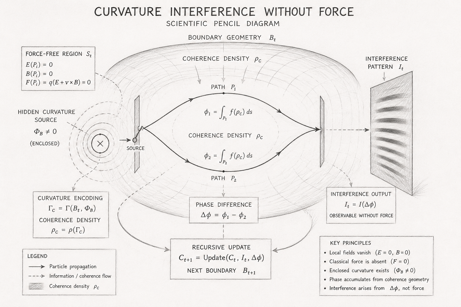
The scientific pencil diagram for Curvature Interference Without Force illustrates one of the central principles of the Holographic Space-Time (HST) framework: that measurable interference phenomena can arise entirely from differences in boundary coherence geometry, even when particles travel through regions where the classical electromagnetic force is absent.

Rather than depicting forces acting upon particles, the diagram visualises the recursive evolution of coherence information encoded within the surrounding boundary.

Every element contributes to a continuous causal chain that begins with hidden curvature and ends with an observable interference pattern.

Overall Structure of the Diagram

The figure is organised as a left-to-right recursive flow representing the evolution of physical information.

The complete sequence is

Boundary Geometry
        ↓
Force-Free Region
        ↓
Hidden Curvature
        ↓
Coherence Curvature
        ↓
Coherence Density
        ↓
Independent Paths
        ↓
Phase Accumulation
        ↓
Phase Difference
        ↓
Interference Pattern
        ↓
Recursive Boundary Update

Unlike a conventional ray diagram, the emphasis is not on forces or field lines but on the gradual accumulation of coherence information along different trajectories.

The Boundary Geometry

The large shaded envelope surrounding the entire experiment represents the evolving boundary

\[ B_t \]

Within HST this boundary is not a physical wall nor a spacetime surface.

Instead, it is the geometric information structure that contains the coherence relationships governing the evolution of the system.

Every subsequent quantity shown in the diagram is derived from this boundary.

The light pencil shading illustrates that coherence is distributed continuously rather than concentrated at isolated points.

The Force-Free Region

On the left of the figure the boxed equations define the force-free propagation region.

The conditions

\[ E(P_i)=0 \]

\[ B(P_i)=0 \]

and

\[ F(P_i)=q(E+v\times B)=0 \]

state that particles experience no measurable local electromagnetic force while travelling through the experiment.

This region is crucial because it establishes that any observed interference cannot be attributed to conventional Lorentz dynamics. The diagram therefore separates the concepts of force and geometric information, making clear that the latter alone is sufficient to produce observable effects within the HST interpretation.

The Hidden Curvature Source

The concentric circular structure at the left of the diagram represents the enclosed curvature source,

\[ \Phi_B \]

The source is shown outside the particle trajectories because it does not act locally on the particles. Instead, it modifies the surrounding boundary geometry, producing a coherent curvature distribution throughout the entire region.

The concentric rings symbolise curvature encoded within the boundary rather than electromagnetic field lines. They indicate that structural information extends beyond the immediate location of the enclosed source and influences the geometry sampled by every possible path.

Curvature Encoding

Immediately below the source, the diagram introduces the transformation

\[ \Gamma_C=\Gamma(B_t,\Phi_B) \]

followed by

\[ \rho_C=\rho(\Gamma_C) \]

These equations describe the conversion of hidden boundary curvature into a continuous coherence density.

Within the HST framework, this is the mechanism by which geometric information becomes physically accessible. The coherence density does not exert a force; instead, it defines the informational landscape through which particles propagate. This transformation is one of the key conceptual advances illustrated by the diagram.

The Coherence Density Field

The softly shaded interior of the boundary, labelled

\[ \rho_C \]

represents the continuous distribution of coherence density.

Unlike classical field diagrams that show discrete vectors, the shading indicates a smoothly varying informational medium. The density is continuous across the region, emphasising that coherence is a distributed property of the boundary rather than a localised interaction.

This continuous landscape provides the structural environment sampled by every particle trajectory.

The Two Independent Paths

The upper and lower curves,

\[ P_1 \]

and

\[ P_2 \]

represent two independent force-free trajectories through the same coherence field.

Although both particles experience identical classical conditions, each path traverses a different portion of the coherence landscape. Consequently, each accumulates a unique geometric history.

The divergence and later convergence of the paths visually reinforce the idea that different coherence environments can produce distinct physical outcomes despite identical local forces.

Phase Accumulation Along Each Path

The equations

\[ \phi_1=\int_{P_1} f(\rho_C)\,ds \]

and

\[ \phi_2=\int_{P_2} f(\rho_C)\,ds \]

are positioned directly beside their respective trajectories.

Their placement indicates that phase is accumulated continuously as the particles move through the coherence density. Every infinitesimal segment contributes to the total coherence history of that path.

Within HST these integrals represent the accumulation of geometric information rather than simply the evolution of a quantum wavefunction.

Phase Difference

The central lower box computes

\[ \Delta\phi=\phi_1-\phi_2 \]

This quantity compares the complete coherence histories of the two trajectories.

Rather than measuring the effect of a force, the phase difference measures the structural distinction between the two encoded paths. It is the first directly observable consequence of differences in boundary geometry.

The diagram places this calculation beneath the trajectories to emphasise that it emerges only after both coherence histories have been completed.

The Interference Pattern

On the right side of the figure the familiar interference fringes appear, labelled

\[ I_t=I(\Delta\phi) \]

The fringes demonstrate that observable interference is generated solely from the accumulated phase difference.

Their location at the end of the diagram reinforces the causal sequence:

boundary geometry → coherence density → path history → phase difference → interference.

The accompanying annotation, "Observable Without Force," summarises the principal conclusion of the chapter: measurable interference can arise even though the particles encounter no local electromagnetic force during propagation.

Recursive Boundary Update

At the bottom of the figure the recursion box introduces

\[ C_{t+1}=\operatorname{Update}(C_t,I_t,\Delta\phi) \]

This stage extends the interpretation beyond a single measurement.

The interference result is incorporated into the evolving coherence state, which then contributes to the next boundary configuration,

\[ B_{t+1} \]

The curved feedback arrows illustrate that the system is not static but recursively self-consistent. Every observation becomes part of the evolving coherence geometry that governs future evolution.

The Legend

The legend in the lower-left corner defines the symbolic language of the diagram:

  • Solid arrows represent the physical propagation of particles along their trajectories.
  • Dashed arrows denote the flow of coherence information and recursive structural influence rather than material transport.
  • Shaded regions indicate the continuous coherence density ρC, emphasising that the medium is informational rather than mechanical.

This distinction allows the reader to separate particle motion from the underlying evolution of coherence geometry.

Key Principles Panel

The boxed summary at the lower-right condenses the principal theoretical assumptions illustrated throughout the figure:

  • Local electric and magnetic fields vanish.
  • Classical force remains absent.
  • Hidden boundary curvature persists.
  • Phase accumulates from coherence geometry.
  • Interference is produced by the phase difference rather than by local force.

These statements form the conceptual bridge between the Flow Algebra, the mathematical formulation, and the visual representation.

Scientific Interpretation

Viewed as a whole, the diagram provides a graphical execution trace of the HST model for Curvature Interference Without Force.

It demonstrates that hidden boundary curvature generates a continuous coherence density, that independent force-free paths accumulate different geometric histories while traversing this density, and that their resulting phase difference produces an observable interference pattern.

The recursive update closes the causal loop by feeding the measurement back into the evolving boundary state, illustrating that physical systems within HST are governed by continuous coherence evolution rather than by isolated force interactions.

The figure therefore encapsulates the central claim of the chapter: interference is interpreted not as the consequence of local forces, but as the measurable manifestation of recursively accumulated boundary coherence.

Diagram → Flow Mapping Table

Curvature Interference Without Force

The following table provides a one-to-one correspondence between every major element shown in the scientific pencil diagram and its equivalent component in the Flow Algebra execution model.

This mapping demonstrates how the visual representation, the recursive flow, and the underlying scientific interpretation describe the same physical process from complementary perspectives.

Diagram Element Flow Algebra Component Scientific Function Execution Role
Entire Boundary Envelope B_t = Boundary(t) Defines the evolving coherence geometry of the physical system. Initialises the complete boundary state from which all subsequent quantities are derived.
Force-Free Region Box S_t ⊂ B_t Defines the observation region where particles propagate without measurable classical force. Establishes the valid execution domain for interference analysis.
Electric Field Constraint E(P_i) = 0 Removes local electrostatic interactions from the propagation paths. Verifies force-free conditions.
Magnetic Field Constraint B(P_i) = 0 Removes local magnetic interactions from the propagation paths. Ensures no local Lorentz force exists.
Force Constraint F(P_i) ≤ Ftol Confirms classical forces remain below measurable threshold. Prevents force-driven interference from entering the model.
Hidden Curvature Source Φ_B ≠ 0 Represents enclosed coherence curvature that exists independently of local force. Supplies the structural information required to generate coherence curvature.
Curvature Encoding Box Γ_C = Γ(B_t, Φ_B) Converts boundary geometry into coherent curvature information. Generates the executable coherence structure.
Coherence Density Box ρ_C = ρ(Γ_C) Produces the continuous coherence-density landscape. Creates the informational medium through which particles propagate.
Shaded Boundary Region ρ_C Visualises the spatial distribution of coherence density. Represents the continuous coherence field sampled by every trajectory.
Particle Source Initialise(P_i) Defines the common origin of both propagation paths. Begins recursive particle evolution.
Upper Path P₁ First force-free trajectory through the coherence field. Samples one coherence history.
Lower Path P₂ Second force-free trajectory through the coherence field. Samples an independent coherence history.
Phase Integral on Upper Path φ₁ = ∫P₁ f(ρ_C) ds Accumulates coherence information along Path 1. Computes the first geometric phase.
Phase Integral on Lower Path φ₂ = ∫P₂ f(ρ_C) ds Accumulates coherence information along Path 2. Computes the second geometric phase.
Phase Difference Box Δφ = φ₁ − φ₂ Compares the accumulated coherence histories of both paths. Produces the measurable phase displacement.
Interference Screen I_t = I(Δφ) Displays the observable interference pattern. Converts geometric phase difference into experimental observation.
Recursive Update Box C_{t+1} = Update(C_t, I_t, Δφ) Incorporates the measurement into the evolving coherence state. Updates the recursive system for the next iteration.
Feedback Arrow C_{t+1} → B_{t+1} Demonstrates recursive boundary evolution. Completes one execution cycle and prepares the next.
Solid Arrows → Represent physical particle propagation. Define the execution direction of particle evolution.
Dashed Arrows Recursive Information Transfer Represent coherence influence rather than material transport. Show structural information flowing through the boundary.
Pencil Shading Continuous ρ_C Illustrates smoothly varying coherence density. Indicates that coherence exists as a distributed geometric property rather than discrete force vectors.

Complete Diagram Execution Mapping

Visual Sequence Flow Execution Scientific Meaning
Boundary Geometry B_t The evolving coherence boundary defines the physical system.
Force-Free Region S_t Particle propagation occurs where local electromagnetic forces vanish.
Hidden Curvature Φ_B Enclosed curvature remains encoded despite the absence of local fields.
Curvature Encoding Γ_C = Γ(B_t,Φ_B) Boundary geometry converts enclosed curvature into coherent structure.
Coherence Density ρ_C = ρ(Γ_C) Curvature generates a continuous informational landscape.
Independent Paths P₁, P₂ Multiple trajectories sample different coherence regions.
Phase Accumulation φ₁, φ₂ Each path records its unique geometric coherence history.
Phase Difference Δφ Relative coherence histories become experimentally distinguishable.
Interference Pattern I_t Observable interference emerges from the phase difference rather than local force.
Recursive Update C_{t+1} Measurement updates the evolving coherence geometry for future evolution.

Diagram Logic versus Flow Logic

Diagram Feature Equivalent Flow Statement Interpretation
Outer boundary surrounds every component B_t initialises the complete system All physical evolution occurs within a single coherent boundary.
Curvature source lies outside particle paths Φ_B ≠ 0 Geometry influences propagation without exerting local force.
Two separated trajectories P₁, P₂ Independent coherence histories develop simultaneously.
Different phase integrals φ₁, φ₂ Path-dependent coherence accumulates continuously.
Central phase comparison Δφ = φ₁ − φ₂ Observable differences arise from accumulated geometry.
Fringes on detector I_t = I(Δφ) Interference is the measurable manifestation of coherence differences.
Feedback loop Update(C_t, I_t, Δφ) Every observation contributes recursively to future boundary evolution.

Scientific Interpretation

The mapping table demonstrates that every visual component in the pencil diagram has a direct counterpart within the Flow Algebra.

The boundary envelope corresponds to the evolving coherence geometry, the force-free region enforces the absence of classical interactions, the hidden curvature source generates the coherence landscape, and the independent particle paths accumulate distinct geometric histories.

These histories are compared through the phase difference, producing an interference pattern without invoking local electromagnetic forces.

The recursive update completes the execution cycle by feeding the measurement back into the boundary state, illustrating the central HST principle that physical evolution is governed by continuously evolving coherence geometry rather than isolated force interactions.

The diagram and the Flow Algebra are therefore two complementary representations of the same recursive scientific model: one visual, one formal, both describing interference as the observable consequence of accumulated boundary coherence.

Execution Guarantee Statement

Execution Guarantee

The Curvature Interference Without Force Flow Algebra executes deterministically provided that the physical system satisfies the structural coherence conditions defined throughout the model.

Execution begins by establishing an active boundary geometry BtB_t, within which a force-free propagation region StS_t is identified. The model guarantees that particle evolution is interpreted exclusively through boundary coherence if the local electromagnetic conditions remain

\[ E(P_i)=0 \]

\[ B(P_i)=0 \]

and

\[ F(P_i)\leq F_{\mathrm{tol}} \]

These constraints ensure that no measurable classical Lorentz force contributes to the evolution of either particle trajectory.

Execution proceeds only when a hidden coherence curvature remains enclosed within the boundary,

\[ \Phi_B\neq 0 \]

allowing the boundary to generate a coherent curvature field through

\[ \Gamma_C=\Gamma(B_t,\Phi_B) \]

Provided that the resulting curvature exceeds the minimum structural stability threshold,

\[ \Gamma_C\geq\Gamma_{\min} \]

the boundary produces a continuous coherence density,

\[ \rho_C=\rho(\Gamma_C) \]

which satisfies

\[ \operatorname{Continuity}(\rho_C)=\mathrm{TRUE} \]

The model further guarantees deterministic execution only if both particle trajectories remain mutually coherent throughout propagation,

Coherence(P1​,P2​)≥Cmin​.

Under these conditions each trajectory accumulates a unique coherence phase,

\[ \phi_i=\int_{P_i} f(\rho_C)\,ds \]

and their difference,

\[ \Delta\phi=\phi_1-\phi_2 \]

is computed without ambiguity.

Whenever the accumulated phase satisfies the observational threshold,

\[ \left|\Delta\phi\right|\geq\varepsilon_{\mathrm{phase}} \]

the interference function

\[ I_t=I(\Delta\phi) \]

must produce a stable, measurable interference pattern arising solely from differences in accumulated boundary coherence. Within the scope of this HST model, no local force term is required to generate the observable result.

The recursive update,

\[ C_{t+1}=\operatorname{Update}(C_t,I_t,\Delta\phi) \]

is guaranteed to preserve coherence consistency, ensuring that the updated state becomes the initial boundary condition for the next execution cycle without violating any previously established invariants.

Structural Execution Guarantees

The Flow Algebra guarantees the following throughout successful execution:

  • Boundary Consistency: The evolving boundary remains the single source of coherence geometry.
  • Force-Free Propagation: Local electric fields, magnetic fields, and classical Lorentz forces remain absent along all particle trajectories.
  • Curvature Preservation: Hidden enclosed curvature continues to generate stable coherence geometry throughout execution.
  • Density Continuity: Coherence density remains continuous and free of structural discontinuities.
  • Deterministic Phase Accumulation: Every trajectory accumulates a unique coherence history determined solely by the boundary geometry it traverses.
  • Unique Interference Prediction: The computed phase difference produces one deterministic interference outcome for a given coherence configuration.
  • Recursive Stability: Each completed execution updates the global coherence state while preserving all structural invariants required for subsequent iterations.

Failure Conditions

Execution is intentionally terminated if any of the following conditions occur:

\[ F(P_i)>F_{\mathrm{tol}} \]

indicating that classical forces are no longer negligible;

\[ E(P_i)\neq0\ \lor\ B(P_i)\neq0 \]

showing that local electromagnetic fields are present;

\[ \Phi_B=0 \]

meaning no hidden curvature remains enclosed;

\[ \Gamma_C<\Gamma_{\min} \]

indicating insufficient boundary coherence to sustain stable curvature;

\[ \operatorname{Continuity}(\rho_C)=\mathrm{FALSE} \]

showing a discontinuous coherence landscape;

\[ \operatorname{Coherence}(P_1,P_2)<C_{\min} \]

indicating loss of mutual path coherence; or

\[ \left|\Delta\phi\right|<\varepsilon_{\mathrm{phase}} \]

meaning that the accumulated phase difference is too small to produce a measurable interference pattern.

Under any of these conditions, the recursive execution halts because the structural assumptions of the model are no longer satisfied.


Telephone:
01377 236594

Scientific Guarantee

Within the Holographic Space-Time framework, this Flow Algebra provides a structurally deterministic execution model for curvature-driven interference.

If the boundary geometry remains coherent, the propagation region remains force-free, hidden curvature continues to encode the coherence landscape, and independent trajectories accumulate distinct coherence histories, then the model guarantees that an observable interference pattern will emerge as a direct consequence of recursive boundary coherence.

In this formulation, interference is guaranteed to arise from accumulated geometric information rather than from the direct action of local classical forces, completing the HST interpretation of Curvature Interference Without Force as a fully recursive, coherence-based physical process.

Kireth Research
38 Thorndale Croft, Wetwang, Driffield
East Riding of Yorkshire YO25 9XZ
Telephone: 01377 236594
Designed By