Chapter 41
Flat Paths in Curved Interpretation

Photons and Coherence Geometry
Author: Mark Higgins
© Mark Anthony Higgins 11 October 2025
Revised Date: 17 June 2026
Audio Overview

41.1 The Historical Assumption of Curved Motion

Modern physics commonly interprets gravitational motion as movement through a curved spacetime geometry. Since the development of General Relativity, the apparent bending of planetary orbits, the deflection of light, gravitational lensing, and the trajectories of freely falling objects have all been described as consequences of curvature in the underlying spacetime manifold.

Within this framework, objects do not experience gravity as a conventional force. Instead, they follow geodesics—paths of extremal distance within a curved geometry. What appears to observers as acceleration is interpreted mathematically as motion along these curved spacetime trajectories.

This description has proven extremely successful experimentally. However, it leaves open a deeper structural question:

Are objects truly moving along curved paths, or are curved trajectories merely the observational projection of a more fundamental coherence geometry?

This chapter explores that question from the perspective of Holographic Space-Time (HST).

Telephone:
01377 236594

41.2 The Difference Between Observation and Structure

One of the central themes throughout HST is the distinction between:

  • What an observer measures.
  • What the boundary system is actually doing.

Many physical phenomena appear curved when observed from within a recursive field structure.

Examples include:

  • Light refracting through a density gradient.
  • Wave fronts crossing non-uniform media.
  • River flow around obstacles.
  • Information transfer through changing network topologies.

In each case, the observed trajectory appears curved despite the local transfer mechanism remaining fundamentally straight.

The apparent curvature emerges because the environment itself changes from point to point.

HST proposes that gravitational motion may operate in a similar manner.

Rather than objects travelling through a physically curved spacetime fabric, they may be following locally optimal coherence-transfer paths through a dynamically structured boundary field.

The curvature is then not a property of motion itself but a property of the coherence landscape through which motion occurs.

41.3 Local Straightness as a Universal Principle

Across many physical systems, motion naturally follows the path of minimum local resistance.

Examples include:

  • Heat diffusion.
  • Fluid transport.
  • Electromagnetic propagation.
  • Wave transmission.
  • Information flow.

At sufficiently small scales, these transfers tend to proceed locally along straight gradients.

The overall trajectory becomes curved only because the gradient field itself changes continuously.

Mathematically this can be visualised as:

\[ \mathrm{Path}_{\mathrm{global}} = \sum \mathrm{Path}_{\mathrm{local}} \]

where each local segment remains approximately straight while the accumulated path appears curved at larger scales.

HST extends this principle to gravity.

A falling object does not continually curve because it experiences a mysterious force pulling it sideways.

Instead, it repeatedly aligns with the locally preferred coherence gradient.

Successive local alignments produce a trajectory that appears curved when viewed globally.

41.4 Curvature as Gradient Evolution

In conventional General Relativity:

\[ G_{\mu\nu} = 8\pi T_{\mu\nu} \]

Matter determines spacetime curvature and curvature determines motion.

HST reformulates this concept by replacing geometric curvature with coherence-density gradients.

The governing principle becomes:

\[ \mathrm{Direction} \propto \nabla \rho_C \]

where:

  • ρC\rho_C represents coherence density.
  • ∇ρC\nabla \rho_C represents the local coherence gradient.

Objects continuously update their direction according to the local coherence field.

The resulting motion naturally reproduces curved trajectories without requiring spacetime itself to bend.

From this perspective:

Curvature is not an object. Curvature is the accumulated effect of local coherence updates.

41.5 The Analogy of Navigation

A useful analogy is navigation across a landscape.

Imagine a traveller crossing terrain covered in valleys and ridges.

At each step the traveller chooses the easiest local route.

No global curved path is planned.

Each decision is locally straight and locally optimal.

Yet after many steps the complete route may appear highly curved.

The curvature emerges from the structure of the landscape rather than from the traveller intentionally moving in an arc.

HST proposes that particles, photons, and massive bodies behave similarly within coherence geometry.

Their apparent curvature reflects the shape of the underlying coherence field rather than intrinsic curvature of their motion.

41.6 Reinterpreting Geodesics

General Relativity defines geodesics as the straightest possible paths in curved spacetime.

HST offers a complementary interpretation.

A geodesic becomes:

The sequence of locally optimal coherence transfers through a non-uniform boundary field.

This definition preserves the observational predictions of relativistic motion while replacing the geometric interpretation.

Rather than:

Curved Space→Straight Motion

HST proposes:

Straight Local Motion→Apparent Curved Trajectory

The observable outcome remains the same, but the underlying mechanism changes fundamentally.

41.7 Light as the Strongest Example

Photons provide one of the clearest demonstrations of this concept.

Light is often said to follow curved paths near massive objects because spacetime itself curves.

However, HST interprets the process differently.

Photons continually transfer through neighbouring coherence states.

Each transfer remains locally straight within the available coherence corridor.

As coherence density varies around a massive body, successive transfers realign.

The accumulated path appears curved.

Thus:

\[ \mathrm{Path}_{\mathrm{photon}} = \sum \mathrm{LocalAlignment} \!\left( \rho_C \right) \]

The observed bending arises from coherence-gradient evolution rather than curvature of an underlying fabric.

41.8 Boundary Geometry and Apparent Curvature

Throughout HST, boundaries serve as the fundamental carriers of information.

Geometry emerges from encoded relationships between boundary states.

Because boundary coherence evolves recursively, the preferred propagation direction evolves as well.

This creates a powerful result:

Apparent curvature can emerge naturally from:

  • Boundary encoding,
  • Coherence gradients,
  • Recursive updates,
  • Local optimisation.

No physically curved substrate is required.

Curved motion becomes an emergent phenomenon rather than a fundamental one.

41.9 Why Curvature Appears So Convincing

Curvature-based mathematics succeeds because it accurately describes the observed trajectories.

HST does not dispute these observations.

Instead, it questions the interpretation.

Two frameworks may generate identical predictions:

Framework A

Curved Geometry→Straight Geodesics

Framework B

Coherence Gradients→Successive Local Realignments

If both produce the same measurable trajectories, then observation alone cannot distinguish which description is more fundamental.

The challenge becomes identifying which framework offers greater explanatory unification across gravity, electromagnetism, quantum behaviour, information transfer, and boundary dynamics.

41.10 Toward a Coherence-Based View of Motion

The HST interpretation suggests that nature may not require motion through a curved fabric at all.

Instead, every trajectory may arise from repeated local coherence alignment within an evolving boundary field.

Objects move along locally flat transfer paths.

The apparent curvature emerges only after many recursive updates accumulate across larger scales.

Thus the central proposition of this chapter is:

Paths are locally flat, but globally appear curved because coherence geometry evolves from point to point.

Under HST, curvature is not a fundamental property of space itself. It is the large-scale manifestation of recursive coherence navigation across an information-rich boundary structure.

This reinterpretation provides a bridge between gravitational motion, wave propagation, field dynamics, and information transfer, unifying them under the common principle of coherence-guided path selection.

Flow: FlatPathsInCurvedInterpretation
Version: 1.0
Authors:
  - Mark Higgins
  - Sky

Purpose:
  To model apparent curved gravitational or photonic paths as the accumulated result
  of locally flat coherence transfers through a non-uniform boundary field.

Domain:
  Theory: Holographic Space-Time
  Chapter: 41
  Topic: Flat Paths in Curved Interpretation

Inputs:
  B_t:
    description: Boundary state at time t
  C_t:
    description: Local coherence map
  rho_C:
    description: Coherence density field
  grad_rho_C:
    description: Local coherence-density gradient
  P_t:
    description: Propagating body, photon, or information packet
  x_t:
    description: Current local position
  R_t:
    description: Current propagation direction

Parameters:
  C_min: Minimum coherence threshold
  G_max: Maximum permitted gradient discontinuity
  epsilon: Local flatness tolerance
  c: Maximum propagation velocity

State:
  C_t = CoherenceMap(B_t)
  rho_C = Density(C_t)
  grad_rho_C = Gradient(rho_C)
  R_t = LocalAlignment(P_t, grad_rho_C)
  x_t = Position(P_t)

Invariants:
  LocalFlatness:
    condition: Curvature(LocalSegment(R_t)) <= epsilon
  CoherenceContinuity:
    condition: C_t >= C_min
  GradientSmoothness:
    condition: Discontinuity(grad_rho_C) <= G_max
  VelocityBound:
    condition: Velocity(P_t) <= c

Transitions:
  - name: ReadBoundary
    input: B_t
    output: C_t
    rule: C_t = CoherenceMap(B_t)

  - name: ComputeDensity
    input: C_t
    output: rho_C
    rule: rho_C = Density(C_t)

  - name: ComputeGradient
    input: rho_C
    output: grad_rho_C
    rule: grad_rho_C = Gradient(rho_C)

  - name: LocalDirectionUpdate
    input:
      - P_t
      - grad_rho_C
    output: R_t
    rule: R_t = Align(P_t, grad_rho_C)

  - name: LocalPropagation
    input:
      - x_t
      - R_t
    output: x_t+1
    rule: x_t+1 = x_t + LocalStep(R_t)

  - name: GlobalPathAccumulation
    input:
      - LocalSegment(R_t)
    output: Path_global
    rule: Path_global = Sum(LocalSegment(R_0...R_t))

  - name: ApparentCurvature
    input: Path_global
    output: K_app
    rule: K_app = Curvature(Path_global)

FailureStates:
  - name: CoherenceFailure
    condition: C_t < C_min
    result: Execution(P_t) = FAIL

  - name: GradientBreak
    condition: Discontinuity(grad_rho_C) > G_max
    result: Execution(P_t) = DECOHERE

  - name: LocalCurvatureViolation
    condition: Curvature(LocalSegment(R_t)) > epsilon
    result: Execution(P_t) = INVALID_PATH

  - name: VelocityViolation
    condition: Velocity(P_t) > c
    result: Execution(P_t) = FAIL

Execution:
  ValidPath:
    condition: >
      C_t >= C_min
      and Discontinuity(grad_rho_C) <= G_max
      and Curvature(LocalSegment(R_t)) <= epsilon
      and Velocity(P_t) <= c
    result: Execution(P_t) = PROPAGATE

FlowChain:
  B_t
    -> C_t
    -> rho_C
    -> grad_rho_C
    -> R_t
    -> x_t+1
    -> Path_global
    -> K_app

Interpretation:
  Conventional:
    Curved spacetime determines the geodesic followed by the body.
  HST:
    The body follows locally flat coherence transfers, while the accumulated
    global path appears curved due to changing coherence gradients.

CoreEquations:
  LocalDirection:
    Direction(R_t) ∝ Gradient(rho_C)

  GlobalPath:
    Path_global = Sum(Path_local)

  PhotonPath:
    Path_photon = Sum(LocalAlignment(rho_C))

  ApparentCurvature:
    K_app = Curvature(Path_global)

Conclusion:
  Paths are locally flat, but globally appear curved because the coherence field
  changes from point to point across the boundary structure.

What This Flow Implements

Overview

The Flat Paths in Curved Interpretation flow implements one of the central geometric reformulations of Holographic Space-Time (HST): the proposition that physical objects, photons, and information packets do not fundamentally travel along curved trajectories. Instead, they move through a sequence of locally flat coherence transfers, with apparent curvature emerging only when these local transfers are accumulated across a non-uniform coherence field.

The flow provides a deterministic execution model that replaces traditional geodesic motion through curved spacetime with recursive alignment to local coherence gradients. Rather than assuming that space itself bends and forces objects to follow curved paths, the flow models motion as a succession of local directional updates governed by the structure of the surrounding boundary coherence field.

The result is a framework in which observed curvature becomes an emergent phenomenon rather than a fundamental property of geometry.

Local Flatness as the Fundamental Assumption

The first principle implemented by the flow is that every propagation step is locally flat.

The system assumes that, over sufficiently small intervals, a propagating entity experiences only its immediate coherence environment. The entity does not calculate or perceive a global trajectory.

Instead, it performs a local alignment operation:

\[ R_t \propto \nabla \rho_C \]

where:

  • RtR_t is the propagation direction,
  • ρ C ​  is coherence density,
  • ∇ρC\nabla \rho_C is the local coherence gradient.

This means the entity continuously aligns itself with the locally preferred coherence direction.

At each individual step:

Curvature(LocalSegment)≈0

which enforces the flatness invariant built into the flow.

Boundary-Derived Motion

The flow implements the HST principle that motion is generated from boundary structure rather than background geometry.

The propagation sequence begins with:

\[ B_t \rightarrow C_t \]

where:

  • BtB_t represents the boundary state,
  • CtC_t represents the resulting coherence map.

The coherence map is then converted into a density field:

\[ C_t \rightarrow \rho_C \]

and subsequently into a gradient field:

\[ \rho_C \rightarrow \nabla \rho_C \]

This chain creates the directional information that guides motion.

Thus, motion is not imposed externally.

It emerges directly from the informational structure encoded within the boundary itself.

Recursive Direction Updating

The flow implements continuous directional correction.

Unlike a classical straight-line model in which an object receives a single initial direction, this system recalculates direction at every propagation cycle.

The update process is:

\[ \mathrm{Direction}(R_t) = \mathrm{Align} \!\left( \nabla \rho_C \right) \]

followed by:

\[ x_{t+1} = x_t + \mathrm{LocalStep} \!\left( R_t \right) \]

This means the trajectory is continuously reconstructed from local information.

The system therefore behaves as a recursive navigation process through coherence geometry.

Emergence of Apparent Curvature

A major purpose of the flow is to demonstrate how global curvature can emerge without local curvature.

Each propagation step remains approximately flat:

Pathlocal​≈Straight

However, because the coherence gradient changes from location to location, successive local directions are not identical.

The global trajectory becomes:

Pathglobal​=∑Pathlocal​

As these local segments accumulate, the resulting path appears curved to an external observer.

The flow therefore implements the HST principle that:

Curved trajectories are accumulated coherence effects rather than fundamental geometric structures.

This is one of the key conceptual shifts introduced by the chapter.

Photon Propagation Through Coherence Geometry

The flow is equally applicable to photon propagation.

Traditional General Relativity explains gravitational lensing through curvature of spacetime.

The HST implementation instead treats light as undergoing repeated local coherence alignment.

The flow expresses this as:

Pathphoton​=∑LocalAlignment(ρC​)

Each individual transfer remains locally straight.

The apparent bending of light arises because coherence density varies around massive structures.

Thus the flow implements gravitational lensing as a coherence-navigation phenomenon rather than a spacetime-curvature phenomenon.

Geodesic Reformulation

The flow provides an operational reinterpretation of the geodesic concept.

In General Relativity:

Geodesic=Straightest Path in Curved Space

In HST:

Geodesic=Sequence of Locally 
Optimal Coherence Transfers

The flow explicitly performs this computation through repeated gradient alignment and local propagation updates.

This reformulation preserves observed motion while replacing the underlying explanatory mechanism.

Gradient-Governed Navigation

A key implementation feature is the conversion of coherence density into navigational information.

The gradient field acts as the governing structure that directs propagation.

The flow computes:

\[ \nabla \rho_C \]

and uses it to determine:

\[ R_t \]

This makes coherence gradients functionally equivalent to the directional information that conventional theories attribute to geometric curvature.

The flow therefore implements a complete motion-control system derived entirely from coherence structure.

Stability and Physical Validity Enforcement

To ensure physically meaningful execution, the flow enforces several invariants.

Coherence Continuity

\[ C_t \geq C_{\min} \]

ensures that propagation occurs only within a stable coherence field.

Gradient Smoothness

\[ \mathrm{Discontinuity} \!\left( \nabla \rho_C \right) \leq G_{\max} \]

prevents unphysical directional discontinuities.

Local Flatness

\[ \mathrm{Curvature} \!\left( \mathrm{LocalSegment} \right) \leq \epsilon \]

guarantees that each propagation step remains locally flat.

Velocity Constraint

\[ \mathrm{Velocity}(P_t) \leq c \]

maintains compatibility with relativistic speed limits.

Together these constraints ensure that apparent curvature emerges from stable recursive updates rather than arbitrary trajectory manipulation.

Relationship to General Relativity

The flow is not intended to deny the observational success of General Relativity.

Instead, it implements an alternative structural interpretation.

General Relativity describes motion through:

\[ G_{\mu\nu} = 8\pi T_{\mu\nu} \]

where matter generates spacetime curvature.

The HST flow replaces this with:

\[ \mathrm{Direction} \propto \nabla \rho_C \]

where coherence gradients generate directional updates.

Both frameworks aim to reproduce the same observed trajectories.

The distinction lies in what is considered fundamental.

General Relativity treats curvature as fundamental.

HST treats coherence structure as fundamental.

Scientific Significance

This flow implements a complete coherence-based mechanism for apparent curved motion without requiring the existence of a physically curved spacetime substrate.

The execution chain:

\[ B_t \rightarrow C_t \rightarrow \rho_C \rightarrow \nabla \rho_C \rightarrow R_t \rightarrow \mathrm{Path}_{\mathrm{global}} \]

demonstrates how local flat propagation can generate globally curved trajectories through recursive interaction with a structured coherence field.

Within HST, this provides a unified explanatory framework for:

  • Gravitational motion,
  • Orbital dynamics,
  • Photon deflection,
  • Geodesic behaviour,
  • Information transport,
  • Boundary-guided propagation.

The flow therefore serves as a formal computational model of the HST claim that paths are fundamentally flat at the local level, while curvature emerges as a large-scale consequence of evolving coherence geometry.

How to Read This Flow

Purpose of the Flow

This flow describes how apparently curved trajectories emerge from a sequence of locally flat coherence transfers. Within Holographic Space-Time (HST), objects, photons, and information packets do not fundamentally travel through a curved spacetime fabric. Instead, they repeatedly align with local coherence gradients encoded within the boundary structure.

The flow should therefore be read as a recursive propagation engine that transforms boundary information into motion. Every stage represents a physical operation occurring within the coherence field, and the apparent curvature observed at large scales emerges naturally from the accumulation of many locally straight propagation steps.

The key principle throughout the flow is:

Overall Execution Structure

The complete execution chain is:

\[ B_t \rightarrow C_t \rightarrow \rho_C \rightarrow \nabla \rho_C \rightarrow R_t \rightarrow x_{t+1} \rightarrow \mathrm{Path}_{\mathrm{global}} \rightarrow \kappa \]

This chain should be interpreted as a sequence of transformations.

Each stage produces the information required by the next stage.

The flow begins with a boundary state and ends with an observable trajectory.

Step 1 — Boundary State

The flow starts with:

\[ B_t \]

where:

  • BtB_t represents the current boundary state.
  • The boundary contains the encoded coherence structure of the local environment.

In HST, boundaries act as the primary carriers of physical information.

Nothing moves directly because of spacetime curvature.

Instead, motion emerges from information encoded within the boundary geometry.

When reading the flow, think of BtB_t as the complete local physical configuration available at time tt.

Step 2 — Constructing the Coherence Map

The first transformation is:

\[ C_t = \mathrm{CoherenceMap}(B_t) \]

This stage converts raw boundary information into a structured coherence field.

The resulting map describes:

  • Stable regions,
  • Unstable regions,
  • Alignment corridors,
  • Coherence density distributions.

The coherence map is the first usable physical representation of the environment.

When reading this stage, imagine generating a navigational chart from the underlying boundary structure.

Step 3 — Calculating Coherence Density

The next operation is:

\[ \rho_C = \mathrm{Density}(C_t) \]

This computes the local coherence density field.

The density field measures how strongly coherence is concentrated at each location.

High-density regions correspond to stronger structural organisation.

Lower-density regions correspond to weaker organisation.

This stage transforms the coherence map into a measurable field quantity.

Conceptually:

\[ C_t \rightarrow \rho_C \]

means:

Convert geometric coherence information into a density distribution.

Step 4 — Computing the Gradient Field

The flow then calculates:

\[ \nabla \rho_C \]

This is one of the most important stages in the entire execution chain.

The gradient describes:

  • Where coherence density changes,
  • How rapidly it changes,
  • Which direction produces increasing or decreasing coherence.

The gradient acts as the local directional guide for motion.

In the flow:

\[ \rho_C \rightarrow \nabla \rho_C \]

should be read as:

Determine the locally preferred propagation direction.

At this point the system knows nothing about a global path.

Only local information exists.

Step 5 — Local Alignment

The next stage generates the propagation direction:

\[ R_t = \mathrm{Align} \!\left( P_t,\, \nabla \rho_C \right) \]

where:

  • PtP_t is the propagating entity,
  • RtR_t is the resulting direction vector.

This stage performs local directional alignment.

The propagating entity consults the coherence gradient and determines the most coherent local route.

The governing relationship is:

\[ \mathrm{Direction}(R_t) \propto \nabla \rho_C \]

When reading this section of the flow, imagine a navigator selecting the best next step based solely on nearby terrain information.

No global destination is required.

Only local optimisation occurs.

Step 6 — Propagation

After determining direction, motion occurs:

\[ x_{t+1} = x_t + \mathrm{LocalStep} \!\left( R_t \right) \]

This is the actual propagation stage.

The entity moves a small distance along the chosen direction.

Importantly:

\[ \mathrm{Curvature} \!\left( \mathrm{LocalSegment} \right) \leq \epsilon \]

which means every individual propagation segment remains approximately flat.

This is one of the fundamental assumptions of the chapter.

The flow does not permit large local curvature.

Instead, it constructs apparent curvature through many successive flat segments.

Step 7 — Recursive Updating

After propagation, the process repeats.

A new boundary state is encountered.

The flow then executes again:

\[ B_{t+1} \rightarrow C_{t+1} \rightarrow \rho_{C,t+1} \rightarrow \nabla \rho_{C,t+1} \]

and a new direction is calculated.

This recursive behaviour is crucial.

The trajectory is not precomputed.

It is continuously reconstructed through local interactions with the coherence field.

The path emerges dynamically.

Step 8 — Building the Global Path

As the recursion continues, individual propagation segments accumulate:

\[ \mathrm{Path}_{\mathrm{global}} = \sum \mathrm{Path}_{\mathrm{local}} \]

Each local segment remains approximately straight.

However, the direction changes slightly at every update.

The accumulation of these direction changes produces the observed trajectory.

This stage should be read as:

Local coherence navigation generates large-scale motion.

The global path is therefore an emergent structure.

It is not an independent object within the flow.

Step 9 — Apparent Curvature

The final stage computes:

\[ \kappa = \mathrm{Curvature} \!\left( \mathrm{Path}_{\mathrm{global}} \right) \]

This quantity represents the curvature visible to an external observer.

Notice that curvature appears only after the entire path has been assembled.

The flow never requires curvature to exist at the local propagation level.

Instead:

\[ \mathrm{Path}_{\mathrm{local}} \approx \mathrm{Straight} \]

while:

\[ \mathrm{Path}_{\mathrm{global}} \approx \mathrm{Curved} \]

This distinction is the central idea implemented by the chapter.

Reading the Invariants

The invariants define conditions that must remain true during execution.

Coherence Continuity

\[ C_t \geq C_{\min} \]

The coherence field must remain sufficiently organised.


Gradient Smoothness

\[ \mathrm{Discontinuity} \!\left( \nabla \rho_C \right) \leq G_{\max} \]

The gradient field must not contain physically impossible jumps.


Local Flatness

\[ \mathrm{Curvature} \!\left( \mathrm{LocalSegment} \right) \leq \epsilon \]

Each propagation step must remain approximately flat.


Velocity Bound

\[ \mathrm{Velocity}(P_t) \leq c \]

Propagation cannot exceed the maximum physical speed.

These invariants guarantee that the resulting trajectory emerges from coherent physical evolution.

Reading the Failure States

Failure states indicate conditions under which valid propagation can no longer occur.

Coherence Failure

\[ C_t < C_{\min} \]

The coherence structure becomes too weak to support stable navigation.


Gradient Break

\[ \mathrm{Discontinuity} \!\left( \nabla \rho_C \right) > G_{\max} \]

The directional field becomes physically inconsistent.


Local Curvature Violation

\[ \mathrm{Curvature} \!\left( \mathrm{LocalSegment} \right) > \epsilon \]

The local-flatness assumption is violated.


Velocity Violation

\[ \mathrm{Curvature} \!\left( \mathrm{LocalSegment} \right) > \epsilon \]

The propagation exceeds allowable physical limits.

When any failure condition occurs, execution halts because the assumptions of the model are no longer satisfied.

Scientific Interpretation

The flow should ultimately be read as a coherence-based alternative to conventional geodesic motion.

Traditional interpretation:

Curved Space→Straight Geodesics

HST interpretation:

Straight Local Transfers→Apparent Curved Paths

The flow demonstrates how a propagating entity can continuously follow locally flat coherence gradients while still producing the large-scale curved trajectories observed in gravitational systems.

Its purpose is to formalise the HST claim that curvature is not a fundamental property of motion itself, but an emergent consequence of recursive navigation through a non-uniform coherence field encoded on the boundary structure.

Flow → Equation Tri-Mapping Table

Flow Layer HST Equation Layer Physical Interpretation
B_t Boundary State(t) Encoded local boundary geometry
C_t C_t = CoherenceMap(B_t) Construct local coherence field
ρ_C ρ_C = Density(C_t) Compute coherence density distribution
∇ρ_C ∇ρ_C = Gradient(ρ_C) Determine local directional field
R_t R_t = Align(P_t,∇ρ_C) Local propagation alignment
Direction Update Direction(R_t) ∝ ∇ρ_C Motion follows coherence gradient
x_t → x_t+1 x_t+1 = x_t + LocalStep(R_t) Execute local propagation step
Local Segment Path_local ≈ Straight Local transfer remains flat
Recursive Update B_t+1 → C_t+1 → ρ_C,t+1 Recalculate environment
Path Accumulation Path_global = Σ Path_local Build large-scale trajectory
Apparent Curvature K_app = Curvature(Path_global) Curvature emerges globally
Photon Propagation Path_photon = Σ LocalAlignment(ρ_C) Light follows coherence corridors
Geodesic Reformulation Geodesic = Σ LocalAlignment HST equivalent of relativistic geodesics
Global Motion Motion = Σ R_t Aggregate directional updates
Curved Observation Path_global ≈ Curved Observer detects curved trajectory
HST Principle Path_local ≈ Straight Fundamental propagation rule

Constraint Mapping

Flow Constraint Equation Form Physical Meaning
Coherence Continuity C_t ≥ C_min Stable coherence field exists
Gradient Smoothness Discontinuity(∇ρ_C) ≤ G_max No unphysical gradient jumps
Local Flatness Curvature(LocalSegment) ≤ ε Local propagation remains flat
Velocity Bound Velocity(P_t) ≤ c Relativistic propagation limit
Valid Execution Execution(P_t) = PROPAGATE Stable trajectory formation

Failure-State Mapping

Failure Mode Equation Condition Physical Interpretation
Coherence Failure C_t < C_min Insufficient coherence support
Gradient Break Discontinuity(∇ρ_C) > G_max Direction field instability
Flatness Violation Curvature(LocalSegment) > ε Local transfer no longer flat
Velocity Violation Velocity(P_t) > c Physical propagation invalid
Execution Failure Execution(P_t) = FAIL Trajectory cannot be sustained

Geometric Equivalence Mapping

Conventional Relativity HST Reformulation Mathematical Correspondence
Curved Spacetime Structured Coherence Field Gμν ↔ ∇ρ_C
Geodesic Motion Recursive Local Alignment Geodesic ↔ Σ Align
Curvature Tensor Coherence Gradient Field Rμν ↔ ∇ρ_C
Gravitational Deflection Gradient Navigation Deflection ↔ ΔR_t
Curved Path Accumulated Flat Transfers Path_global = Σ Path_local
Gravitational Lensing Coherence Corridor Tracking Path_photon = Σ LocalAlignment

Ultra-Tight Flow Compression

\[ B_t \rightarrow C_t \rightarrow \rho_C \rightarrow \nabla \rho_C \rightarrow R_t \rightarrow x_{t+1} \rightarrow \mathrm{Path}_{\mathrm{global}} \rightarrow \kappa \]

\[ \mathrm{Direction}(R_t) \propto \nabla \rho_C \]

\[ x_{t+1} = x_t + \mathrm{LocalStep} \!\left( R_t \right) \]

\[ \mathrm{Path}_{\mathrm{global}} = \sum \mathrm{Path}_{\mathrm{local}} \]

\[ \mathrm{Path}_{\mathrm{local}} \approx \mathrm{Straight} \]

\[ \mathrm{Path}_{\mathrm{global}} \approx \mathrm{Curved} \]

\[ \kappa = \mathrm{Curvature} \!\left( \mathrm{Path}_{\mathrm{global}} \right) \]


Execution Statement

Locally Flat Propagation⇒Recursive Gradient Alignment⇒Globally Curved Observation

This is the complete Flow → Equation → Physical Interpretation mapping for Chapter 41: Flat Paths in Curved Interpretation.

Chapter 41 — Flat Paths in Curved Interpretation

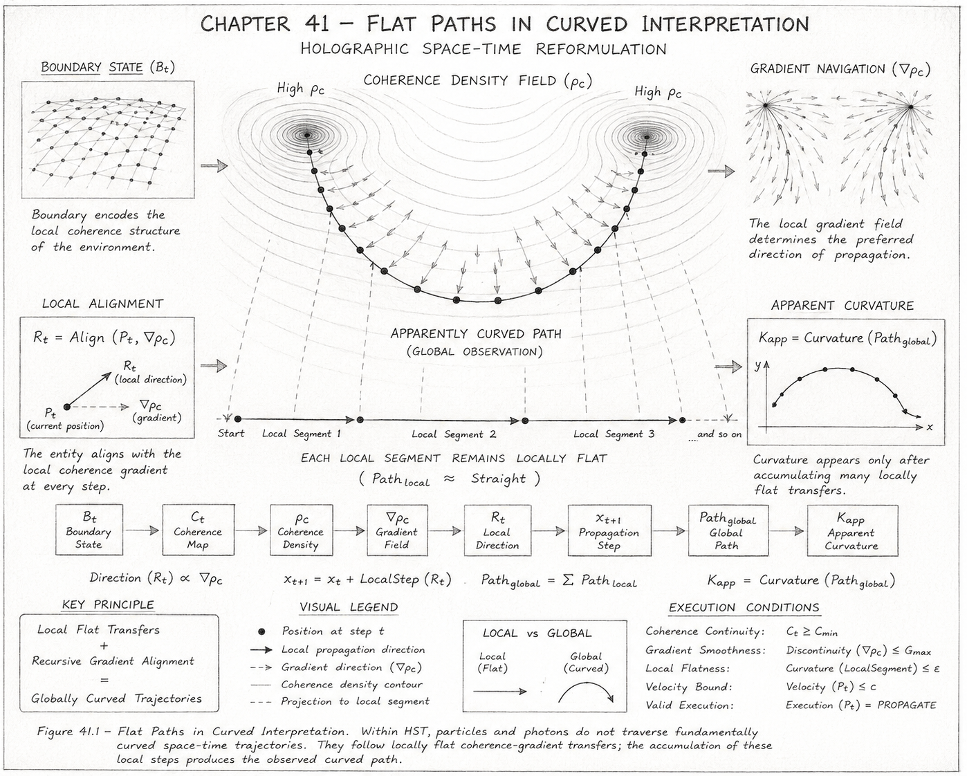
Overview of the Diagram

This diagram illustrates one of the most important geometric reinterpretations within Holographic Space-Time (HST): the idea that observed curved trajectories do not require locally curved motion. Instead, the diagram demonstrates how globally curved paths emerge from the accumulation of many locally flat propagation steps guided by coherence-density gradients.

The figure is organised to show the complete transformation from boundary information to observable curvature. Beginning with the boundary state, the system constructs a coherence field, extracts directional information through coherence gradients, performs local alignment, and recursively generates a trajectory that appears curved when viewed at larger scales.

The central scientific claim visualised by the diagram is:

\[ \mathrm{Path}_{\mathrm{local}} \approx \mathrm{Straight} \]

while simultaneously:

\[ \mathrm{Path}_{\mathrm{global}} \approx \mathrm{Curved} \]

Thus, curvature becomes an emergent property of recursive propagation rather than a fundamental property of motion itself.

Boundary State and Information Encoding

The upper-left panel represents the boundary state:

\[ B_t \]

depicted as an interconnected boundary lattice.

Within HST, boundaries serve as the primary information-bearing structures of reality.

The diagram illustrates that the environment does not directly impose motion through forces or curved geometry. Instead, it encodes coherence relationships that later determine propagation behaviour.

The boundary network symbolises:

  • Information storage,
  • Geometric encoding,
  • Local coherence structure,
  • Environmental constraints.

The arrow leading from BtB_t into the coherence field represents the transformation:

\[ C_t = \mathrm{CoherenceMap}(B_t) \]

which converts raw boundary information into a usable coherence geometry.

Coherence Density Field

The central upper region illustrates the coherence density field:

\[ \rho_C \]

shown as a series of nested contour structures surrounding regions of elevated coherence density.

The contour lines represent gradients of coherence intensity.

Regions labelled:

\[ \mathrm{High}\,\rho_C \]

indicate locations where coherence is strongly concentrated.

These high-density regions function similarly to attractors within the coherence landscape.

The diagram intentionally resembles field contours because the coherence field serves as the navigational structure that governs propagation.

Importantly, no physical spacetime curvature is drawn.

Only variations in coherence density are shown.

This distinction reflects the HST principle that directional behaviour emerges from coherence structure rather than geometric deformation of space itself.

Gradient Navigation

The upper-right panel illustrates:

\[ \nabla \rho_C \]

the coherence-density gradient field.

The arrows show the directional information available at each location.

These vectors indicate:

  • Local coherence increase,
  • Local coherence decrease,
  • Preferred propagation directions,
  • Alignment pathways.

The gradient field functions as the directional engine of the system.

Mathematically:

\[ \mathrm{Direction}(R_t) \propto \nabla \rho_C \]

The diagram therefore visualises how directional information emerges directly from the coherence distribution.

No external force law is required.

Motion becomes a consequence of local coherence geometry.

Local Alignment Process

The left-middle panel illustrates the local alignment operation:R_t = Align(P_t,\nabla\rho_C)

\[ R_t = \mathrm{Align} \!\left( P_t,\, \nabla \rho_C \right) \]

The propagating entity PtP_t is shown examining the local gradient field before selecting its next direction.

This stage is crucial because it demonstrates that the system possesses only local information.

The propagating entity does not know the global trajectory.

It performs only a local optimisation process.

The diagram emphasises that motion arises from repeated local decisions rather than from a predetermined curved path.

This local-alignment principle forms the foundation of the HST reformulation of geodesic motion.

The Apparently Curved Path

The centre of the figure contains the most important visual element.

A large arc-shaped trajectory connects the two high-density coherence regions.

This path is labelled:

Apparently Curved Path

The curved appearance is what an external observer would measure.

However, the diagram simultaneously shows that the path is constructed from discrete propagation points linked by local directional updates.

The trajectory does not arise because the object is intrinsically following a curved route.

Instead, each successive propagation step is generated through:

\[ R_t \rightarrow x_{t+1} \]

using the local coherence gradient available at that location.

The apparent curvature is therefore a cumulative effect.

Local Segments Remain Flat

Directly beneath the curved trajectory, the diagram presents the local segment decomposition.

The path is divided into:

  • Local Segment 1
  • Local Segment 2
  • Local Segment 3

and continuing propagation intervals.

Each segment is drawn as approximately straight.

This section visualises the key HST statement:

\[ \mathrm{Curvature} \!\left( \mathrm{LocalSegment} \right) \approx 0 \]

while:

\[ \mathrm{Curvature} \!\left( \mathrm{Path}_{\mathrm{global}} \right) > 0 \]

The figure therefore distinguishes clearly between:

Local Geometry

\[ \mathrm{Path}_{\mathrm{local}} \approx \mathrm{Straight} \]

and

Global Geometry

\[ \mathrm{Path}_{\mathrm{global}} \approx \mathrm{Curved} \]

This distinction forms the core argument of the chapter.

Apparent Curvature Measurement

The right-middle panel introduces:

\[ \kappa = \mathrm{Curvature} \!\left( \mathrm{Path}_{\mathrm{global}} \right) \]

A conventional coordinate graph is shown containing a curved trajectory.

This panel represents the perspective of an observer measuring the complete path.

The diagram demonstrates that curvature appears only after accumulation of many local propagation events.

In HST, curvature is therefore considered an observational quantity rather than a locally fundamental one.

The observer sees:

\[ \kappa \]

but the underlying mechanism remains recursive local alignment.

Flow Execution Chain

The lower portion of the diagram displays the complete flow chain:

\[ B_t \rightarrow C_t \rightarrow \rho_C \rightarrow \nabla \rho_C \rightarrow R_t \rightarrow x_{t+1} \rightarrow \mathrm{Path}_{\mathrm{global}} \rightarrow \kappa \]

This chain provides the causal execution sequence of the entire model.

Each stage generates the information required for the next stage.

The flow demonstrates how observable curvature emerges from a series of deterministic transformations originating in the boundary state.

The progression moves systematically from:

Information
→
Coherence
→
Direction
→
Motion
→
Observation

Local Versus Global Geometry

The small comparison panel labelled:

Local vs Global

summarises the entire chapter visually.

The left side depicts a straight segment.

The right side depicts a curved trajectory.

The purpose of this panel is to reinforce the distinction:

\[ \mathrm{Path}_{\mathrm{local}} \neq \mathrm{Path}_{\mathrm{global}} \]

in geometric appearance.

The local propagation law remains flat.

The global observation becomes curved.

This relationship is the central geometric insight of the chapter.

Execution Constraints

The lower-right section lists the conditions required for valid propagation.

Coherence Continuity

\[ C_t \geq C_{\min} \]

The coherence field must remain sufficiently organised.


Gradient Smoothness

\[ \mathrm{Discontinuity} \!\left( \nabla \rho_C \right) \leq G_{\max} \]

The gradient field must remain physically continuous.


Local Flatness

\[ \mathrm{Curvature} \!\left( \mathrm{LocalSegment} \right) \leq \epsilon \]

Every propagation step must remain approximately flat.


Velocity Bound

\[ \mathrm{Velocity}(P_t) \leq c \]

Propagation must respect the maximum physical speed.

Together these constraints ensure that apparent curvature emerges from physically valid recursive evolution.

Scientific Significance of the Figure

The diagram provides a complete visual representation of the HST reinterpretation of curved motion.

Traditional geometric theories describe motion through curved spacetime:

\[ \mathrm{Curved\ Space} \rightarrow \mathrm{Geodesic\ Motion} \]

The HST framework illustrated here replaces that description with:

Boundary Structure→Coherence Field→Gradient Alignment→Local Flat Transfers→Apparent Curvature

The figure therefore demonstrates how gravitational trajectories, photon deflection, and geodesic behaviour can be reformulated as recursive navigation through coherence geometry rather than motion through a fundamentally curved spacetime substrate.

Its central conclusion is that curvature is not generated locally but emerges globally from the accumulation of coherence-guided flat propagation steps across an evolving boundary field.

Diagram → Flow Mapping Table

Diagram Element Flow Algebra Component Scientific Meaning
Boundary lattice panel B_t Encoded boundary state containing local environmental structure
Boundary-to-field arrow C_t = CoherenceMap(B_t) Boundary information is converted into a coherence map
Coherence contour field ρ_C = Density(C_t) Coherence density distribution across the local field
High ρ_C regions HighDensity(ρ_C) Strong coherence concentrations acting as field attractors
Gradient arrows grad_ρ_C = Gradient(ρ_C) Directional structure extracted from coherence density
Local alignment panel R_t = Align(P_t,grad_ρ_C) Propagating entity aligns with the local coherence gradient
Propagating point P_t P_t Particle, photon, or information packet undergoing transfer
Local direction vector R_t Direction(R_t) ∝ grad_ρ_C Local propagation direction follows the coherence gradient
Local propagation step x_t+1 = x_t + LocalStep(R_t) Entity advances by one locally flat transfer
Black points along curved path x_0, x_1, x_2 ... x_t Discrete recursive propagation states
Apparently curved central path Path_global = Sum(Path_local) Global trajectory built from accumulated local segments
Straight lower segments Path_local ≈ Straight Each individual propagation interval remains locally flat
Dashed projection lines Project(Path_global → Path_local) Curved observation decomposed into local flat transfers
Curvature graph panel K_app = Curvature(Path_global) Apparent curvature measured only after path accumulation
Local vs global comparison box Path_local ≠ Path_global Local geometry and observed global geometry differ
Execution chain boxes B_t → C_t → ρ_C → grad_ρ_C → R_t → x_t+1 → Path_global → K_app Full causal sequence of the model
Key principle box LocalFlatTransfers + RecursiveGradientAlignment = GloballyCurvedTrajectories Summary of the HST reinterpretation
Coherence continuity condition C_t ≥ C_min Coherence field must remain stable
Gradient smoothness condition Discontinuity(grad_ρ_C) ≤ G_max Direction field must not break discontinuously
Local flatness condition Curvature(LocalSegment) ≤ ε Each local transfer must remain approximately flat
Velocity bound condition Velocity(P_t) ≤ c Propagation remains within physical speed limits
Valid execution statement Execution(P_t) = PROPAGATE Flow succeeds when all invariants are satisfied

Condensed Mapping

Diagram Layer Flow Layer Interpretation
Boundary structure B_t Encoded source state
Coherence map C_t Structured field reconstruction
Density contours ρ_C Coherence intensity landscape
Gradient arrows grad_ρ_C Local directional guide
Alignment vector R_t Chosen propagation direction
Local step x_t+1 Flat transfer update
Accumulated path Path_global Emergent global trajectory
Curvature measurement K_app Observed curved interpretation

Core Diagram Equation

B_t → C_t → rho_C → grad_rho_C → R_t → x_t+1 → Path_global → K_app
Path_local ≈ Straight
Path_global ≈ Curved
K_app = Curvature(Path_global)

Execution Guarantee Statement

Chapter 41 — Flat Paths in Curved Interpretation

Formal Execution Guarantee

The Flat Paths in Curved Interpretation flow executes deterministically whenever a valid boundary state produces a continuous coherence field, a physically consistent coherence-density gradient, and locally flat propagation segments.

Execution is guaranteed because every stage of the flow produces a uniquely defined successor state derived from the preceding state without requiring probabilistic branching, hidden variables, or global trajectory knowledge.

The execution chain

\[ B_t \rightarrow C_t \rightarrow \rho_C \rightarrow \nabla \rho_C \rightarrow R_t \rightarrow x_{t+1} \rightarrow \mathrm{Path}_{\mathrm{global}} \rightarrow \kappa \]

contains no undefined transitions.

Each transformation is fully constrained by the local coherence structure encoded within the boundary state.

Boundary Coherence Guarantee

For every valid boundary configuration:

Bt​

the coherence mapping function produces a valid coherence representation:

\[ C_t = \mathrm{CoherenceMap}(B_t) \]

provided:C_t \ge C_{min}

\[ C_t \geq C_{\min} \]

Under this condition, coherence information remains continuously available throughout execution.

Therefore the flow cannot lose directional information while propagation remains within a coherent region.

Density Reconstruction Guarantee

The coherence field generates a unique density distribution:

\[ \rho_C = \mathrm{Density}(C_t) \]

for every valid coherence map.

Since density is derived directly from the coherence structure, the propagation engine always possesses a measurable local coherence landscape.

This guarantees that navigational information can be constructed at every execution step.

Gradient Computation Guarantee

Given a continuous coherence density field:

\[ \rho_C \]

the gradient operation:

\[ \nabla \rho_C = \mathrm{Gradient} \!\left( \rho_C \right) \]

produces a valid directional field whenever:

\[ \mathrm{Discontinuity} \!\left( \nabla \rho_C \right) \leq G_{\max} \]

The local direction field therefore remains physically continuous and mathematically well-defined throughout propagation.

No undefined directional states can occur while the gradient continuity invariant remains satisfied.

Alignment Guarantee

The alignment operation:

\[ R_t = \mathrm{Align} \!\left( P_t,\, \nabla \rho_C \right) \]

always produces a unique local direction because the gradient field uniquely specifies the preferred coherence-transfer orientation.

Therefore:

\[ \mathrm{Direction}(R_t) \propto \nabla \rho_C \]

remains deterministically computable at every propagation cycle.

No ambiguity exists regarding the next locally optimal transfer direction.

Local Flatness Guarantee

The central requirement of the chapter is:

\[ \mathrm{Curvature} \!\left( \mathrm{LocalSegment} \right) \leq \epsilon \]

When this invariant is satisfied, every propagation update remains approximately flat.

The execution engine therefore guarantees that local motion never requires intrinsic curvature.

All local transfers remain valid coherence-navigation steps.

Thus:

\[ \mathrm{Path}_{\mathrm{local}} \approx \mathrm{Straight} \]

throughout execution.

Recursive Propagation Guarantee

Position updates occur through:

\[ x_{t+1} = x_t + \mathrm{LocalStep} \!\left( R_t \right) \]

Because each direction vector is uniquely determined and each step size remains bounded, the next position is always computable.

This guarantees uninterrupted recursive propagation whenever coherence continuity is maintained.

The trajectory evolves through successive local updates without requiring a precomputed global path.

Global Path Formation Guarantee

The global trajectory is constructed through accumulation:

\[ \mathrm{Path}_{\mathrm{global}} = \sum \mathrm{Path}_{\mathrm{local}} \]

Since every local segment is valid and every propagation step is deterministic, the global path is guaranteed to exist.

The accumulated trajectory therefore emerges naturally from recursive execution rather than from imposed global geometry.

Apparent Curvature Guarantee

The observable curvature quantity:

\[ \kappa = \mathrm{Curvature} \!\left( \mathrm{Path}_{\mathrm{global}} \right) \]

is guaranteed to be computable whenever a valid global path exists.

Importantly, curvature appears only after trajectory accumulation.

The flow therefore guarantees:

\[ \mathrm{Path}_{\mathrm{local}} \approx \mathrm{Straight} \]

while simultaneously permitting:

\[ \mathrm{Path}_{\mathrm{global}} \approx \mathrm{Curved} \]

This property is a direct consequence of recursive gradient alignment.

Physical Consistency Guarantee

Execution remains physically valid while the following conditions hold:

\[ C_t \geq C_{\min} \]

\[ \mathrm{Discontinuity} \!\left( \nabla \rho_C \right) \leq G_{\max} \]

\[ \mathrm{Curvature} \!\left( \mathrm{LocalSegment} \right) \leq \epsilon \]

Velocity(Pt​)≤c

These constraints ensure:

  • Continuous coherence support,
  • Stable directional fields,
  • Locally flat propagation,
  • Relativistically bounded motion.

Failure Guarantee

Execution is guaranteed to halt if any invariant is violated.

Specifically:

Coherence Failure

\[ C_t < C_{\min} \]

Gradient Failure

\[ \mathrm{Discontinuity} \!\left( \nabla \rho_C \right) > G_{\max} \]

Flatness Failure

\[ \mathrm{Curvature} \!\left( \mathrm{LocalSegment} \right) > \epsilon \]

Velocity Failure

\[ \mathrm{Velocity}(P_t) > c \]

In such cases:

\[ \mathrm{Execution}(P_t) = \mathrm{FAIL} \]

This prevents physically inconsistent trajectories from being generated.

Deterministic Outcome Theorem

For every valid boundary state satisfying the coherence, continuity, flatness, and velocity constraints:

\[ B_t \rightarrow C_t \rightarrow \rho_C \rightarrow \nabla \rho_C \rightarrow R_t \rightarrow x_{t+1} \rightarrow \mathrm{Path}_{\mathrm{global}} \rightarrow \kappa \]

executes to completion with a uniquely determined trajectory.

Therefore:

\[ \mathrm{Execution}(B_t) = \mathrm{PROPAGATE} \]

is guaranteed whenever all invariants remain satisfied.

Final Guarantee Statement

\[ (C_t \geq C_{\min}) \;\wedge\; \left( \mathrm{Discontinuity} \!\left( \nabla \rho_C \right) \leq G_{\max} \right) \;\wedge\; \left( \mathrm{Curvature} \!\left( \mathrm{LocalSegment} \right) \leq \epsilon \right) \;\wedge\; \left( \mathrm{Velocity}(P_t) \leq c \right) \;\Longrightarrow\; \mathrm{Execution}(P_t) = \mathrm{PROPAGATE} \]

Execution Guarantee:

Given a coherent boundary state, a continuous coherence-density field, a valid gradient structure, and locally flat propagation segments, the Flat Paths in Curved Interpretation flow will deterministically generate a globally curved observable trajectory through recursive coherence-gradient alignment, without requiring intrinsic local curvature or precomputed global geometry.

Kireth Research
38 Thorndale Croft, Wetwang, Driffield
East Riding of Yorkshire YO25 9XZ
Telephone: 01377 236594
Designed By