Chapter 31
Stable Curvature Knots

This flow implements the Holographic Space-Time (HST) principle that stable physical structures arise from self-sustaining curvature configurations rather than from static objects existing within a pre-defined spacetime framework.

The model describes how information becomes organised into coherent structures, how those structures generate curvature, and how curvature feeds back into future information states to create a self-reinforcing recursive loop. When this loop remains stable across successive updates, a persistent curvature knot emerges.

In conventional physics, stable particles and matter are often described as entities whose persistence results from force balances, conserved quantities, or energy minima. The Stable Curvature Knots flow reformulates this idea in coherence terms.

Rather than asking why an object remains stable, the flow asks whether the underlying recursive curvature pattern can continuously reconstruct itself.

If the pattern successfully regenerates through each recursion cycle, the structure persists.

If the recursive regeneration fails, the structure gradually dissolves.

The flow begins with an information state:

\[ I_t \]

This information is transformed into an organised coherence map:

\[ I_t \rightarrow C_t \]

The coherence map represents the structured relationships within the information system.

At this stage, no stable object exists yet.

The system merely contains organised informational structure capable of producing higher-order geometry.

The flow next computes coherence density:

\[ \rho_C = \operatorname{density}(C_t) \]

As coherence becomes concentrated, geometric effects emerge.

The model represents this through curvature generation:

\[ \rho_C \rightarrow K_t \]

Curvature is therefore treated as an emergent consequence of coherence density rather than a property of an underlying spacetime fabric.

Within HST, curvature becomes the observable manifestation of organised information.

Curvature alone does not guarantee persistence.

The curvature must remain confined within a stable boundary system:

\[ (K_t, B_t) \rightarrow K_B \]

The boundary constrains the curvature pattern and prevents immediate dispersion.

This creates a finite geometric structure capable of maintaining identity through time.

The resulting configuration forms the basis of a Stable Curvature Knot.

The defining feature of the flow is recursive closure.

Curvature feeds back into future information states:

\[ K_B \rightarrow I_{t+1} \]

The updated information state then regenerates coherence:

\[ I_{t+1} \rightarrow C_{t+1} \]

which regenerates curvature:

\[ C_{t+1} \rightarrow K_{t+1} \]

This produces the self-sustaining loop:

\[ I_t \rightarrow C_t \rightarrow K_t \rightarrow I_{t+1} \rightarrow C_{t+1} \rightarrow K_{t+1} \]

A stable knot exists when this loop continually reconstructs its own geometry.

The flow defines stability through four conditions:

\[ C_t \geq C_{\min} \]

\[ K_t \geq K_{\min} \]

\[ B_t = \mathrm{continuous} \]

\[ \operatorname{Drift}(K_t) \leq R_{\max} \]

These conditions ensure that:

Only when all four conditions are satisfied does the curvature knot remain stable.

Within the flow, matter is reinterpreted as long-lived curvature closure.

Particles become minimal curvature knots.

Atomic systems become coupled knot structures.

Macroscopic objects become large recursive networks of interconnected knots.

The apparent permanence of matter is therefore not a consequence of static existence but of continuous recursive reconstruction.

Existence itself becomes a process rather than a state.

The Stable Curvature Knots flow describes how persistent physical structures emerge from recursive coherence rather than from static matter existing inside a fixed spacetime background.

The flow should be read from top to bottom, following the transformation of information into coherence, coherence into curvature, and curvature into a self-sustaining recursive structure.

The central idea is that stability is not a property that objects possess automatically. Stability emerges when a curvature pattern can continuously regenerate itself through recursive information feedback.

The flow starts with the information state:

\[ I_t \]

This represents all encoded relationships present within the system at recursive step $t$.

Examples may include:

At this stage there is no stable curvature knot.

There is only information available for organisation.

Read:

\[ I_t \]

The first transformation is:

\[ I_t \rightarrow C_t \]

where:

\[ C_t = \operatorname{CoherenceMap}(I_t) \]

This means the system organises information into a structured coherence pattern.

The coherence map represents how well information components align and reinforce one another.

Read:

\[ C_t \]

as:

"The organised coherence structure generated from information."

The flow then calculates coherence density:

\[ \rho_C = \operatorname{density}(C_t) \]

This quantity measures how concentrated the coherence structure has become.

Higher coherence density corresponds to stronger organisation and greater structural persistence.

Read:

\[ \rho_C \]

as:

"The concentration of coherence within the system."

The next transformation is:

\[ \rho_C \rightarrow K_t \]

where:

\[ K_t = \operatorname{Curvature}(\rho_C) \]

In HST, curvature emerges from organised coherence rather than from a pre-existing geometric fabric.

The greater the coherence concentration, the stronger the resulting curvature structure.

Read:

\[ K_t \]

as:

"The curvature geometry generated by coherence density."

The curvature is then constrained by the system boundary:

\[ (K_t, B_t) \rightarrow K_B \]

This step prevents unrestricted geometric dispersion.

The boundary acts as a containment mechanism that allows coherent curvature to remain localised.

Read:

\[ K_B \]

as:

The defining feature of the flow occurs here:

\[ K_B \rightarrow I_{t+1} \]

The curvature structure influences the next information state.

Rather than simply existing, the curvature actively shapes future system evolution.

Read:

\[ I_{t+1} \]

as:

The updated information regenerates coherence:

\[ I_{t+1} \rightarrow C_{t+1} \]

which regenerates curvature:

\[ C_{t+1} \rightarrow K_{t+1} \]

This forms the recursive closure loop:

\[ I_t \rightarrow C_t \rightarrow \rho_C \rightarrow K_t \rightarrow K_B \rightarrow I_{t+1} \rightarrow C_{t+1} \rightarrow K_{t+1} \]

Read this loop as:

"Information creates curvature, curvature modifies information, and the cycle continuously regenerates itself."

This loop is the foundation of a Stable Curvature Knot.

The flow then evaluates four invariants:

\[ C_t \geq C_{\min} \]

The coherence structure must remain sufficiently organised.

\[ K_t \geq K_{\min} \]

Curvature must remain observable.

\[ B_t = \mathrm{continuous} \]

The boundary must remain intact.

\[ \operatorname{Drift}(K_t) \leq R_{\max} \]

Recursive deformation must remain bounded.

These conditions determine whether the knot remains stable.

A Stable Curvature Knot can fail in several ways.

\[ C_t < C_{\min} \]

The structure loses organisation.

\[ K_t < K_{\min} \]

Curvature becomes too weak to remain observable.

\[ B_t = \mathrm{broken} \]

The knot loses confinement.

Excessive Drift

\[ \operatorname{Drift}(K_t) > R_{\max} \]

The geometry evolves too far from its original structure.

Any of these conditions can destabilise the knot.

The master stability condition is:

Stable_Knot⟺(Ct​≥Cmin​)∧(Kt​≥Kmin​)∧(Bt​=continuous)∧(Drift(Kt​)≤Rmax​)

Read this as:

"A Stable Curvature Knot exists if coherence remains organised, curvature remains observable, boundaries remain intact, and recursive deformation remains controlled."

The flow proposes that matter is not fundamentally a collection of static objects.

Instead:

Particle→Curvature Knot

and

\[ \mathrm{Matter} \propto \sum \mathrm{Stable\_Knots} \]

Particles, atoms, molecules, and larger structures are interpreted as self-maintaining recursive curvature configurations.

The persistence of matter therefore becomes a consequence of successful recursive coherence preservation.

In simple terms, this flow describes how a geometric structure can continually rebuild itself through recursive information feedback, allowing stable physical objects to exist as long-lived curvature knots within the HST framework.

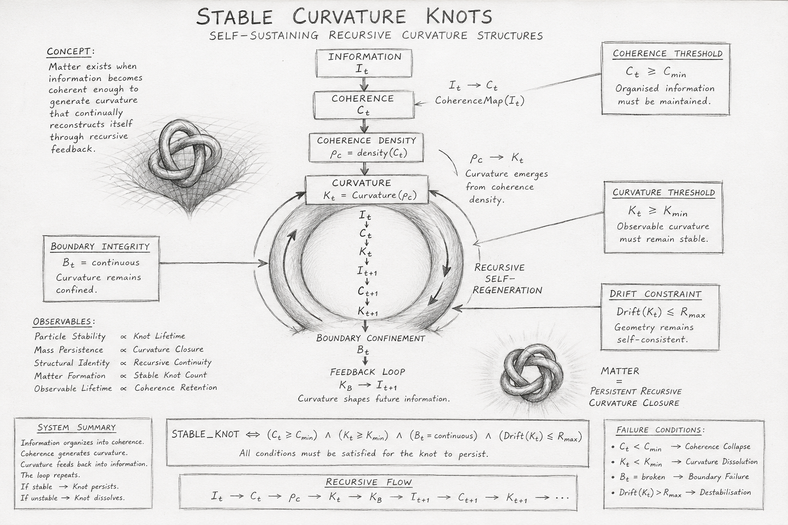
This diagram illustrates the Holographic Space-Time (HST) interpretation of stable physical structures as self-sustaining curvature knots. Rather than treating matter as a collection of permanent objects embedded within a fixed spacetime background, the diagram depicts matter as a continuously regenerated curvature configuration maintained through recursive coherence feedback.

The central idea is that stable existence emerges when a curvature pattern repeatedly reconstructs itself through successive information updates. Persistence therefore becomes a dynamic process of recursive self-maintenance rather than a static property of matter.

The diagram begins at the top with the information state:

\[ I_t \]

This represents the complete informational configuration of the system at recursion step $t$.

As information becomes organised, a coherence structure forms:

\[ I_t \rightarrow C_t \]

The coherence map $C_t$ describes how informational components align into a structured and internally consistent pattern.

This stage represents the emergence of order from information.

The coherence structure produces a measurable coherence density:

\[ \rho_C = \operatorname{density}(C_t) \]

The diagram shows this density feeding into the curvature generation stage:

\[ \rho_C \rightarrow K_t \]

Within HST, curvature is not imposed upon spacetime. Instead, curvature emerges naturally from organised coherence.

As coherence density increases, geometric structure becomes observable.

The resulting curvature configuration is represented by:$${\mathrm{<span\; style="font-family:\; -apple-system,\; BlinkMacSystemFont,\; \text{'}Segoe\; UI\text{'},\; Roboto,\; \text{'}Helvetica\; Neue\text{'},\; Arial,\; \text{'}Noto\; Sans\text{'},\; sans-serif,\; \text{'}Apple\; Color\; Emoji\text{'},\; \text{'}Segoe\; UI\; Emoji\text{'},\; \text{'}Segoe\; UI\; Symbol\text{'},\; \text{'}Noto\; Color\; Emoji\text{'};\; font-size:\; 1rem;"></span>}}_{}$$

\[ K_t \]

which forms the geometric foundation of the Stable Curvature Knot.

At the centre of the diagram sits the recursive knot structure.

This knot represents a curvature geometry that has become sufficiently organised to maintain itself through recursive feedback.

Unlike a static object, the knot is continually regenerated.

The circular arrows illustrate the principle that the structure is self-reinforcing.

The knot survives because each recursion cycle recreates the curvature configuration responsible for its existence.

The diagram therefore portrays stability as an active process rather than passive persistence.

Inside the knot appears the recursive sequence:

It​→Ct​→Kt​→It+1​→Ct+1​→Kt+1​

This sequence represents recursive closure.

Information generates coherence.

Coherence generates curvature.
Curvature influences future information.

The cycle then repeats.

If the regenerated curvature remains sufficiently similar to the previous curvature, the knot persists.
This feedback loop forms the mechanism through which matter maintains long-term stability.

Below the knot the diagram introduces boundary confinement:

Bt​

The boundary acts as a coherence container.

Without confinement, curvature would disperse and the structure would lose stability.

The diagram therefore shows curvature existing within a protected geometric region capable of maintaining recursive organisation.

The confinement condition is represented by:

Bt​=continuous

which indicates that boundary integrity remains intact.

Surrounding the knot are four stability constraints.

Coherence Threshold

\[ C_t \geq C_{\min} \]

The coherence structure must remain sufficiently organised.

If coherence falls below this threshold, the knot loses its internal structure.

\[ K_t \geq K_{\min} \]

Observable curvature must remain present.

If curvature weakens excessively, the knot can no longer maintain physical identity.

\[ B_t = \mathrm{continuous} \]

The boundary must remain unbroken.

A fragmented boundary allows coherence leakage and destabilisation.

\[ \operatorname{Drift}(K_t) \leq R_{\max} \]

The curvature geometry must not deviate excessively between recursion cycles.

Excessive drift prevents successful self-regeneration.

The lower-left section of the diagram lists observable properties that emerge from Stable Curvature Knots.

Particle stability increases with knot lifetime.

Mass persistence increases with curvature closure.

Structural identity emerges from recursive continuity.

Matter formation results from the accumulation of stable knots.

Observable lifetime scales with coherence retention.

These relationships connect the abstract recursive model to measurable physical phenomena.

The lower-right section illustrates the conditions under which a knot ceases to exist.

\[ C_t < C_{\min} \]

Curvature Dissolution

\[ K_t < K_{\min} \]

Observable geometry disappears.​

Confinement is lost.

\[ \operatorname{Drift}(K_t) > R_{\max} \]

The structure evolves beyond its ability to self-reconstruct.

Any of these failures terminate the recursive closure process.

The diagram summarises one of the fundamental claims of HST:

Matter=Persistent Recursive Curvature Closure

In this interpretation, particles, atoms, molecules, and larger structures are not static entities.

They are stable recursive curvature knots whose coherence structure continually regenerates itself through information feedback.

The persistence of matter therefore emerges not from permanence, but from successful recursive self-reconstruction.

Existence becomes a process of continual geometric renewal, maintained by coherence, curvature, boundaries, and recursive closure.

This flow guarantees a deterministic method for evaluating whether a recursive curvature structure can persist as a Stable Curvature Knot within the Holographic Space-Time (HST) framework.

The execution does not assume the existence of stable matter beforehand.

Instead, stability emerges only if the recursive coherence and curvature conditions remain satisfied throughout execution.

The flow therefore provides a formal test for persistent geometric existence.

For every valid input state:

It​

the flow executes the following sequence:

It​→Ct​→ρC​→Kt​→KB​→It+1​

where:

Because every transformation possesses a defined successor state, execution remains deterministic.

A Stable Curvature Knot is guaranteed to exist if and only if all stability invariants remain true:

\[ C_t \geq C_{\min} \]

\[ K_t \geq K_{\min} \]

\[ B_t = \mathrm{continuous} \]

\[ \operatorname{Drift}(K_t) \leq R_{\max} \]

If these conditions are maintained during recursive execution, the curvature geometry continuously regenerates itself.

Therefore:

\[ \mathrm{Structure}_{t+1} \approx \mathrm{Structure}_t \]

and persistence is preserved.

The flow guarantees recursive closure whenever the regenerated curvature remains capable of reconstructing the coherence pattern that produced it.

Formally:

\[ K_t \rightarrow I_{t+1} \rightarrow C_{t+1} \rightarrow K_{t+1} \]

and

\[ K_{t+1} \approx K_t \]

Under this condition the curvature knot remains self-sustaining.

No external stabilisation mechanism is required.

The flow guarantees curvature confinement provided that:

\[ B_t = \mathrm{continuous} \]

A continuous boundary prevents coherence leakage and maintains geometric closure.

Therefore:

\[ K_t \subseteq B_t \]

for all valid recursive states.

This guarantees that curvature remains localised rather than dispersing indefinitely.

The flow guarantees immediate detection of instability whenever one or more invariant conditions fail.

\[ C_t < C_{\min} \]

Result:

\[ K_t < K_{\min} \]

Result:​

\[ B_t = \mathrm{broken} \]

Result:

Drift(Kt​)>Rmax​

Result:

No unstable state can be incorrectly classified as stable.

The flow guarantees that observable matter can emerge only through successful recursive curvature preservation.

Formally:

\[ \mathrm{Matter} \propto \sum \mathrm{Stable\_Knots} \]

and

Stable_Knots⟺Recursive Curvature Closure

Thus the existence of matter directly reflects the successful execution of the recursive stability conditions.

Provided the stability conditions remain satisfied:

\[ \mathrm{Structure}_{t+1} \approx \mathrm{Structure}_t \]

the flow guarantees preservation of structural identity across recursive updates.

The knot may evolve internally, but its defining geometric organisation remains intact.

This allows long-lived physical structures to maintain persistence despite continual recursive change.

The Stable Curvature Knots flow executes successfully if and only if:

When these conditions are satisfied:

Execution(St​)=SUCCESS

Stable_Knot=TRUE

Matter=Observable

When any condition fails:

Execution(St​)=FAIL

Stable_Knot=FALSE

Matter=Dissolve

Information→Coherence→Curvature→Boundary Closure→Recursive Regeneration→Stable Curvature Knot

Therefore, the flow guarantees that any structure capable of preserving coherence, curvature, boundary integrity, and bounded recursive drift will persist as a Stable Curvature Knot, while all structures that fail these requirements will eventually dissolve through recursive instability.