Chapter 8
From Equations to Invariants

The Failure of Dimensional Construction
Author: Mark Higgins
© Mark Anthony Higgins 11 October 2025
Revised Date: 14 April 2026

Reconstructing Physical Law as Constraint-Preserving Structure

Modern physics is written in the language of equations. From Newton's Second Law to the field structure of Maxwell's Equations, and the curvature relations of Einstein Field Equations, physical law is traditionally expressed as symbolic equalities linking measurable quantities. These equations are treated as generative rules: given inputs, they produce outputs—positions, fields, energies, probabilities.

However, this framing conceals a deeper structural truth.

Equations do not generate reality. They restrict it.

The Hidden Role of Invariants

Every physical equation implicitly encodes a set of invariants—conditions that must remain true across all valid evolutions of a system. These invariants are not secondary properties; they are the true carriers of physical law.

  • Conservation of energy
  • Conservation of momentum
  • Charge continuity
  • Causality constraints
  • Boundary coherence conditions

These are not derived consequences—they are filtering conditions on what is allowed to exist.

An equation such as:

\[ F = ma \]

does not produce motion. Instead, it excludes all trajectories that violate the invariant relationship between force, mass, and acceleration.

Likewise, Maxwell’s equations do not construct electromagnetic fields—they enforce:

  • ∇⋅B=0\nabla \cdot B = 0 (no magnetic monopoles)
  • ∇⋅E=ρ/ε0\nabla \cdot E = \rho / \varepsilon_0 (charge-field consistency)
  • Dynamic coupling constraints between EE and BB

These are coherence constraints, not generative instructions.

Equations as Boundary Operators

Within the Flow Algebra framework, this distinction becomes explicit.

A physical system is defined as:

\[ S = (I, R, B, K) \]

Where:

  • II— information state
  • RR — transformation rules (candidate evolution generator)
  • BB — boundary constraints
  • KK — invariants (non-negotiable truths)

Evolution proceeds not by direct computation of equations, but by:

\[ E_t = \mathrm{expand}(I_t, R) \]

\[ V_t = \{x \in E_t \mid x \vDash (B \wedge K)\} \]

x∗∈Vt​

Thus, equations are reinterpreted as membership conditions on VtV_t.

They define what survives—not what is produced.

From Computation to Admissibility

This shift reframes physics from:

“Given inputs, compute outputs”

to:

“Given possibilities, eliminate violations”

Reality is not the result of forward calculation—it is the residual of constraint satisfaction.

This aligns physical law with:

  • Constraint systems in mathematics
  • Admissibility conditions in dynamical systems
  • Feasibility regions in optimisation theory

The universe becomes a selection process, not a computation engine.

Why This Matters

The equation-first view leads to several deep limitations:

  • 1. False Generativity
    Equations appear to produce outcomes, masking the fact that invalid states are simply discarded.
  • 2.Hidden Assumptions
    Constraints (e.g., conservation laws) are treated as consequences rather than primary structure.
  • 3.Fragmentation of Theory
    Each domain introduces its own equations, without a unifying mechanism of validity.
  • 4. Breakdown at Extremes
    Singularities, divergences, and non-physical solutions arise when invariant enforcement is incomplete or inconsistent.

Invariant-First Physics

By placing invariants at the foundation:

  • Equations become surface representations of deeper constraints
  • Physical law becomes domain-independent
  • Cross-theory unification emerges naturally as shared invariants
  • Failure modes (e.g., infinities) are recognised as violations of admissibility, not mysteries

In this view:

Physics≡Constraint-Preserving Evolution

Chapter Direction

This chapter formalises the transition from equation-based reasoning to invariant-based structure.

We will:

  • Decompose canonical equations into their invariant cores
  • Reconstruct physical laws as constraint filters within Flow Algebra
  • Show that all valid evolution is equivalent to survival within VtV_t
  • Demonstrate that equations are compressions of admissibility conditions

The goal is not to discard equations—but to reveal their true role.

Core Thesis

Equations do not define reality.
Invariants define reality.
Equations are merely their shadow.

Flow Algebra Specification v1.0
Chapter 8 — From Equations to Invariants

State:
S_t = (I_t, R, B, K)

Where:
I_t = information state at step t
R   = expansion rules
B   = boundary constraints
K   = invariants

Core expansion:
E_t = expand(I_t, R)

Validity filter:
V_t = {x ∈ E_t | x ⊨ (B ∧ K)}

Selection:
x* ∈ V_t
or
x* = argmax_{x ∈ V_t} P(x | I_t, R, B, K)

Update:
I_{t+1} = update(I_t, x*)
S_{t+1} = (I_{t+1}, R, B, K)

Execution:
Execution(S_t) =
{
  S_{t+1}, if V_t ≠ ∅
  FAIL,    if V_t = ∅
}

Invariant primacy:
∀x : x ∈ V_t ⇒ x ⊨ K
K ⇏ derived from R
K ⇏ derived from I
K is fundamental

Equation reinterpretation:
Equation E ≡ Constraint C_E ⊆ (B ∪ K)

Thus:
E ⇏ state generation
E ⇒ state validation

Existence condition:
V_t ≠ ∅ ⇔ coherent physical evolution exists
V_t = ∅ ⇒ FAIL

Invariant enforcement:
∃x ∈ E_t : x ⊭ K      allowed during expansion
x ⊭ K ⇒ x ∉ V_t       never survives

Compression principle:
{E_1, E_2, ..., E_n} ⇒ K_system

Non-generative law:
R generates candidates, not truths
(B ∧ K) selects truths

Failure condition:
V_t = ∅ ⇒ no x* ⇒ no I_{t+1} ⇒ no continuation

Repair modes:
1. Non-fundamental adjustment:
   I_t → I_t'
   or
   R → R'

2. Fundamental repair:
   (B, K) → (B', K')

Derived geometry:
D_t = G(I_t)

D_t ⇏ E_t
D_t ⇏ V_t
D_t ⇏ x*

Closure:
S_t → E_t → V_t → x* → S_{t+1}

Final identity:
Physical Law ≡ Invariant-Constrained State Survival
Equations ≡ Compressed Representations of (B ∧ K)

What This Flow Implements

Invariant-Driven Physical Law as Constraint-Preserving Evolution

1. Recasting Physical Law as a Selection System

This flow implements a non-generative model of physics, in which the evolution of a system is not computed directly from equations, but instead emerges through constraint-based selection over a space of possible states.

Formally, the system evolves via:

\[ S_t \rightarrow E_t \rightarrow V_t \rightarrow x^* \rightarrow S_{t+1} \]

where:

  • EtE_t represents all candidate continuations generated by rules RR
  • VtV_t represents the subset of candidates that satisfy boundary conditions and invariants
  • x∗x^* is a valid continuation selected from VtV_t

This structure implements a fundamental shift:

Reality is not computed — it is filtered.

2. Equations as Embedded Constraints

Within this flow, traditional physical equations are not treated as forward-execution rules. Instead, they are embedded as constraint predicates within the validation layer:

\[ V_t = \{x \in E_t \mid x \vDash (B \wedge K)\} \]

Each equation corresponds to a condition that must evaluate to true for a candidate state xx to remain viable.

For example:

  • Force–acceleration consistency
  • Field divergence constraints
  • Conservation relations

These are implemented as boolean admissibility checks, not computational transformations.

Thus, the flow replaces:

Equation⇒Output

with:

Equation⇒Validity Condition

3. Invariant-Centred Ontology

The flow enforces a strict separation between:

  • Generation (via RR)
  • Validation (via BBand KK)

Here, invariants KK are elevated to primary ontological status:

\[ \forall x^* :\; x^* \vDash K \]

This means:

  • Invariants are always satisfied in any physically realisable state
  • Violations may appear during expansion but are eliminated during validation
  • Physical law is defined by what cannot be violated, not by what is computed

This implements an invariant-first ontology, where:

Existence = survivability under invariant constraints

4. Pre-Physical Expansion Layer

The expansion step:

\[ E_t = \mathrm{expand}(I_t, R) \]

constructs a pre-physical possibility space.

Key properties:

  • It is unconstrained by physical law
  • It may include inconsistent, non-physical, or divergent candidates
  • It is purely generative and structurally unconcerned with validity

This separation is critical: it ensures that validity is not assumed during generation, but instead enforced explicitly afterward.

5. Admissibility as the Mechanism of Reality

The set:

\[ V_t = \{x \mid x \vDash (B \wedge K)\} \]

defines the admissible region of state space.

This flow therefore implements reality as:

  • A feasibility region in a high-dimensional constraint space
  • A survival set under invariant enforcement
  • A coherence manifold defined by non-violation

If:

\[ V_t \neq \emptyset \]

then evolution proceeds.

If:

\[ V_t = \emptyset \]

then:

  • No valid continuation exists
  • The system halts (FAIL)
  • This corresponds physically to inconsistency or breakdown of theory

6. Selection as Resolution of Indeterminacy

When multiple valid states exist:

\[ \lvert V_t \rvert > 1 \]

the flow resolves ambiguity via:

\[ x^* = \arg\max_{x \in V_t} P(x \mid I_t, R, B, K) \]

This introduces:

  • Statistical selection
  • Probabilistic weighting
  • Context-dependent resolution

Importantly:

  • Probability operates within validity, not instead of it
  • Invalid states are never considered, regardless of probability

Thus, the flow cleanly separates:

  • Logical admissibility (hard constraint)
  • Statistical preference (soft selection)

7. Failure as Structural Inconsistency

The condition:

\[ V_t = \emptyset \]

is interpreted as a fundamental failure of coherence.

This implements a powerful diagnostic mechanism:

  • Failure is not numerical error
  • Failure is not approximation breakdown
  • Failure is absence of any admissible state

This corresponds to:

  • Contradictory constraints
  • Incomplete invariant sets
  • Physically impossible configurations

8. Theory Evolution via Constraint Repair

The flow explicitly encodes two modes of response to failure:

Non-Fundamental Adjustment
  • Modify ItI_t or RR
  • Changes representation, not structure
Fundamental Repair
  • Modify (B,K)(B, K)
  • Redefines admissibility itself

This implements scientific theory evolution as:

Adjustment of invariants to restore non-empty admissibility

9. Geometry as a Derived Projection

The mapping:

\[ D_t = G(I_t) \]

defines geometry as a secondary, observational layer.

The flow enforces:

\[ D_t \not\Rightarrow E_t,\quad D_t \not\Rightarrow V_t,\quad D_t \not\Rightarrow x^* \]

Thus, geometry:

  • Does not generate states
  • Does not validate states
  • Does not determine evolution

It is a representation of underlying relational structure, not a causal substrate.

10. Model-Agnostic Physical Execution

Because the flow depends only on:

\[ (I, R, B, K) \]

and not on any specific computational mechanism, it guarantees:

\[ \forall M_1, M_2:\; O_{M_1} = O_{M_2} \]

provided the structure is identical.

This implements:

  • Cross-model consistency
  • Substrate independence
  • Zero-shot executability

Physics becomes a portable constraint system, not an implementation-dependent computation.

11. Compression of Equations into Invariants

Multiple equations:

E1​,E2​,…,En​

are implemented as:

𝐾 system

This flow therefore performs an implicit compression:

  • Reducing symbolic expressions into minimal constraint sets
  • Eliminating redundancy
  • Exposing shared structural dependencies

12. Final Implementation Insight

This flow implements a complete redefinition of physical law:

  • Not as equation execution
  • Not as numerical simulation
  • But as constraint-preserving survival

Formally:

\[ \text{Physics} \equiv \{x \mid x \vDash (B \wedge K)\} \]

evolving through:

Expansion→Filtering→Selection

Closing Statement

This flow does not compute reality.
It enforces the conditions under which reality is allowed to exist.

How to Read This Flow

A Scientific Guide to Interpreting Invariant-Based Physical Structure

1. Read the Flow as a State Evolution System

This flow must be interpreted as a discrete state-transition system, not as a sequence of algebraic manipulations.

At every step, the system is defined as:

\[ S_t = (I_t, R, B, K) \]

This is not a symbolic expression—it is a complete specification of a physical system at time tt.

  • ItI_t: encodes the current informational configuration
  • RR: defines how candidate futures can be generated
  • BB: constrains admissibility within a domain
  • KK: enforces invariant truths across all states
Reading rule:

Treat StS_t as a structured object, not a variable to be solved.

2. Interpret Expansion as Pre-Physical Generation

The step:

\[ E_t = \mathrm{expand}(I_t, R) \]

should be read as:

“Generate all possible continuations permitted by the transformation rules.”

This is not a physical process—it is a logical construction of possibility space.

Key interpretation rules:

  • EtE_t includes invalid and inconsistent states
  • No equation or invariant is enforced here
  • This layer is deliberately unconstrained
Reading rule:

Do not assume anything in EtE_t is physically real.

3. Treat Validation as the Core of Physics

The central operation of the flow is:

\[ V_t = \{x \in E_t \mid x \vDash (B \wedge K)\} \]

This must be read as:

“Filter all candidate states by enforcing boundary conditions and invariants.”

This is the only place where physical law operates.

Interpretation:

  • x⊨(B∧K)x \models (B \wedge K) means state xx satisfies all constraints
  • All physical equations are embedded here as validation conditions
  • Anything not satisfying B∧KB \wedge K is eliminated from reality
Reading rule:

Physics happens at the filtering stage, not during generation.

4. Reinterpret Equations as Constraints

Whenever an equation appears in the theory, it must be read as a membership condition in VtV_t, not as a computational rule.

Example interpretation shift:

  • Traditional reading:
    “Compute acceleration from force and mass.”
  • Flow reading:
    “Reject any state where force and acceleration are inconsistent.”

Thus:

Equation⇒Constraint on x

Reading rule:
Every equation defines what is forbidden, not what is produced.

5. Understand Selection as Resolution, Not Generation

The step:

\[ x^* \in V_t \]

should be read as:

“Choose a valid continuation from the admissible set.”

Important distinctions:

  • The flow does not generate x∗x^* directly
  • It selects x∗x^* from already valid candidates
  • Selection may be deterministic or probabilistic

If:

\[ \lvert V_t \rvert = 1 \]

then:

  • The system is fully constrained
  • Evolution is uniquely determined

If:

\[ \lvert V_t \rvert > 1 \]

then:

Additional selection criteria apply (e.g., probability)

Reading rule:
Selection resolves ambiguity—it does not create structure.

6. Interpret Failure as Physical Impossibility

The condition:

\[ V_t = \emptyset \]

must be read as:

“No physically admissible state exists.”

This is not a computational failure—it is a structural contradiction.

Implications:

  • The system cannot evolve
  • The current configuration violates invariants
  • The theory (or constraints) may be incomplete or inconsistent
Reading rule:
FAIL means reality cannot continue under current constraints.

7. Distinguish Between Generation and Validation

A critical reading discipline is maintaining the separation:

Layer Role
\( R \) Generates possibilities
\( B, K \) Enforces admissibility
\( V_t \) Defines physical reality

Common error to avoid:

Interpreting equations as part of RR

Correct interpretation:

Equations belong to B∧KB \wedge K, not to RR
Reading rule:
Never confuse candidate generation with physical validation.

8. Recognise Geometry as a Derived Representation

The mapping:

\[ D_t = G(I_t) \]

should be read as:

“Construct a geometric representation of the informational state.”

This representation:

  • Does not influence evolution
  • Does not constrain validity
  • Is not part of the physical substrate
Reading rule:
Geometry is descriptive, not causal.

9. Track Invariants Across All Steps

Invariants KK must be mentally carried through every stage of the flow.

For any selected state:

\[ x^* \vDash K \]

This implies:

  • Invariants are never violated in realised states
  • Any apparent violation indicates either:
  • Misinterpretation
  • Incomplete constraint specification
Reading rule:
If an invariant appears broken, the flow has not been correctly applied.

10. Interpret the Flow as Constraint Propagation

The entire structure should be read as a constraint propagation system:

\[ I_t \rightarrow E_t \rightarrow V_t \rightarrow I_{t+1} \]

Where:

  • Constraints propagate forward through filtering
  • Only admissible structure survives
  • Evolution is the preservation of coherence

This aligns the flow with:

  • Constraint satisfaction systems
  • Feasibility filtering in optimisation
  • Logical consistency propagation

11. Read Time as Sequential Constraint Satisfaction

Time progression:

\[ t \rightarrow t+1 \]

should not be interpreted as physical motion through space, but as:

“Sequential resolution of admissibility under invariant constraints.”

Thus:

  • Time is the index of constraint resolution steps
  • Evolution is the preservation of valid structure across steps

12. Final Reading Discipline

To correctly interpret this flow:

  • 1. Start from StS_t as a complete system definition
  • 2. Expand into unconstrained possibilities EtE_t
  • 3. Apply all constraints to obtain VtV_t
  • 4. Select a valid continuation x∗x^*
  • 5. Update the system to St+1S_{t+1}
  • 6. Repeat

At no point should you:

  • Compute outputs directly from equations
  • Assume geometry is fundamental
  • Allow invariant violations to persist

Closing Instruction

Read this flow not as mathematics being executed,
but as structure being tested for survival.

Flow → Equation Tri-Mapping

Flow Layer Flow Algebra Expression Equation Form (Classical) Invariant / Constraint Meaning
System State \( S_t = (I_t, R, B, K) \) State variables \( (x, v, E, B, \rho, \dots) \) Complete physical configuration (non-geometric)
Expansion \( E_t = \text{expand}(I_t, R) \) General solution space / differential evolution space All mathematically possible continuations
Constraint Encoding \( B \wedge K \) Governing equations set \( \{ \mathcal{E}_i \} \) Laws expressed as admissibility conditions
Valid Set \( V_t = \{ x \in E_t \mid x \models (B \wedge K) \} \) Solution set satisfying equations Physically admissible states only
Selection \( x^* \in V_t \) Particular solution / trajectory Realised state consistent with all constraints
Probabilistic Select \( \arg\max P(x \mid I, R, B, K) \) Statistical mechanics / quantum weighting Preference within admissible manifold
Update \( I_{t+1} = \text{update}(I_t, x^*) \) Time evolution \( x(t+\Delta t) \) State progression preserving invariants
Execution \( S_t \rightarrow S_{t+1} \) Integration of equations over time Sequential constraint-preserving evolution
Failure \( V_t = \varnothing \Rightarrow \text{FAIL} \) No solution / divergence / inconsistency Constraint violation → no physical continuation

Canonical Equation → Constraint Mapping

1. Mechanics (Force Law)
Equation Flow Interpretation
\( F = ma \) \( C_{F=ma}(x): \text{force–acceleration consistency must hold} \)

\[ x \in V_t \;\Rightarrow\; F(x) - m(x)a(x) = 0 \]

2. Electromagnetism (Field Constraints)
Equation Flow Constraint Form
\( \nabla \cdot B = 0 \) \( C_B(x): \text{magnetic divergence-free condition} \)
\( \nabla \cdot E = \rho / \varepsilon_0 \) \( C_E(x): \text{charge-field consistency} \)

\[ x \in V_t \;\Rightarrow\; \nabla \cdot B(x) = 0 \]

\[ x \in V_t \;\Rightarrow\; \nabla \cdot E(x) - \frac{\rho(x)}{\varepsilon_0} = 0 \]

3. Conservation Laws (Invariant Set KK)
Law Flow Constraint Form
Energy conservation \( C_E(x): \lvert E'(x) - E(x) \rvert \le \epsilon \)
Momentum conservation \( C_p(x): p_{\text{total}} = \text{const} \)
Charge conservation \( \partial_t \rho + \nabla \cdot J = 0 \)

\[ x \in V_t \;\Rightarrow\; K(x) = \text{true} \]

4. General Structure

All equations reduce to:

\[ E_i(x) = 0 \;\Longrightarrow\; C_i(x) = \text{true} \]

\[ x \in V_t \;\Leftrightarrow\; \forall i,\; E_i(x) = 0 \]


Equation → Flow Collapse

\[ \{E_1, E_2, \ldots, E_n\} \;\Longrightarrow\; (B \wedge K) \]

\[ V_t = \{x \mid \forall i,\; E_i(x) = 0\} \]

Execution Identity (Tri-Equivalent Form)

Flow Form

\[ S_t \rightarrow E_t \rightarrow V_t \rightarrow x^* \rightarrow S_{t+1} \]

Equation Form

\[ \text{Solve } \{E_i(x) = 0\} \]

Invariant Form

\[ x^* \vDash (B \wedge K) \]

Ultra-Compressed Scientist Mapping

\[ E_t \equiv \text{solution space (unconstrained)} \]

\[ V_t \equiv \text{solution space satisfying } E_i \]

\[ x^* \equiv \text{selected valid solution} \]

\[ E_i \equiv \text{constraint filters on } x \]

\[ \text{Physics} \equiv \{x \mid E_i(x) = 0\} \]

Final Equivalence Statement

\[ \text{Solving Equations} \equiv \text{Filtering Candidates by Invariants} \] \[ \text{Equations} \equiv \text{Constraint Operators on } E_t \] \[ \text{Reality} \equiv V_t \]

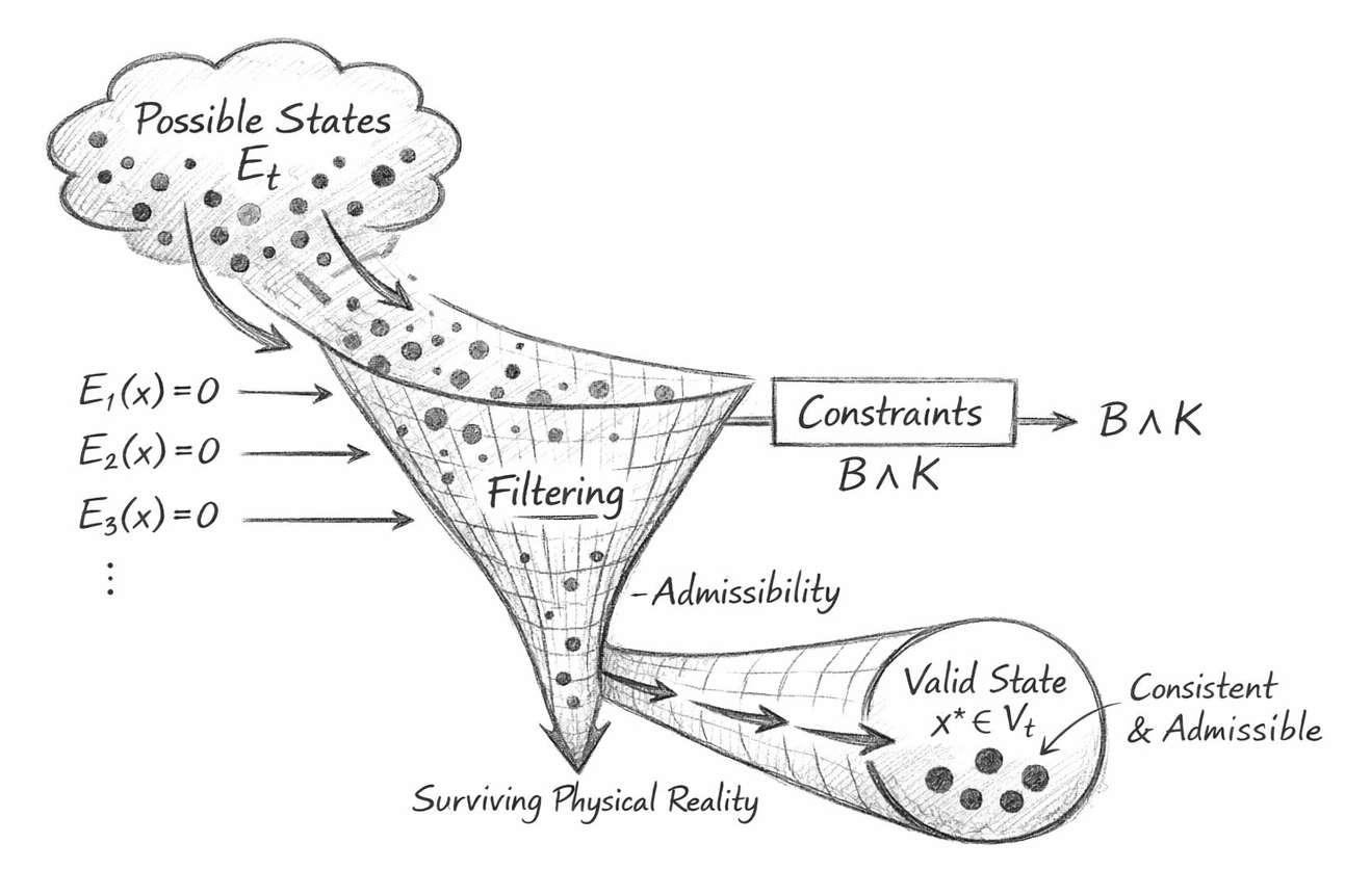
Equation → Constraint → Valid State Funnel

1. Overview of the Diagram Structure

The diagram presents a funnel-based representation of physical law, illustrating the transformation from an unconstrained space of possibilities to a single admissible physical state.

It encodes the full Flow Algebra pipeline:

\[ S_t \rightarrow E_t \rightarrow V_t \rightarrow x^* \rightarrow S_{t+1} \]

but expressed geometrically as a progressive constraint filtration system.

2. Upper Region — Pre-Physical Possibility Space (EtE_t)

The cloud-like structure at the top represents:

\[ E_t = \mathrm{expand}(I_t, R) \]

This region contains:

  • All candidate states generated from the current information state
  • Both physically valid and invalid configurations
  • No enforcement of equations or invariants

The scattered points inside this region denote:

Unfiltered state candidates, including inconsistent, divergent, or non-physical configurations.

Interpretation:

This layer corresponds to the mathematical solution space prior to constraint enforcement, not to physical reality itself.

3. Lateral Inputs — Equations as Constraint Operators

The set of expressions:

\[ E_1(x)=0,\; E_2(x)=0,\; E_3(x)=0,\; \ldots \]

are shown entering the funnel laterally.

This placement is deliberate and encodes a critical reinterpretation:

  • Equations do not act along the main flow
  • They are not used to generate states
  • They act as external constraint filters

Each equation defines a predicate:

\[ C_i(x) \coloneqq \big(E_i(x) = 0\big) \]

Collectively forming:

\[ B \wedge K \]

Interpretation:

Equations function as admissibility tests, not evolution rules.

4. Funnel Body — Constraint Filtering

The narrowing funnel represents the operation:

\[ V_t = \{x \in E_t \mid x \vDash (B \wedge K)\} \]

Within this region:

  • Candidate states are progressively eliminated
  • Only those satisfying all constraints survive
  • The density of points decreases as violations are removed

The visual narrowing encodes:

  • Increasing constraint enforcement
  • Reduction of admissible degrees of freedom
  • Convergence toward a coherence manifold
Interpretation:

This stage is the core of physical law, where invariants and boundaries enforce consistency.

5. Throat Region — Admissibility Boundary

The narrowest point of the funnel represents the condition:

\[ x \vDash (B \wedge K) \]

This is the critical boundary of physical existence.

At this point:

  • All surviving states satisfy every constraint
  • All violations have been removed
  • The system reaches full coherence

If no state reaches this point:

\[ V_t = \emptyset \Rightarrow \mathrm{FAIL} \]

Interpretation:

The throat defines the existence condition of reality under the current constraint set.

6. Lower Channel — Surviving Physical Reality

Below the throat, the diagram shows a narrowed channel labeled:

Surviving Physical Reality

This region corresponds to:

\[ V_t \]

It contains:

  • Only invariant-preserving states
  • Only physically admissible configurations
  • The reduced manifold of valid evolution paths

The transition from wide funnel to narrow channel encodes:

Reality as a strict subset of possibility.

7. Terminal Node — Selected State (x∗∈Vtx^* \in V_t)

At the end of the flow, a single cluster is shown:

\[ x^* \in V_t \]

This represents:

  • The realised physical state
  • A specific admissible continuation
  • The outcome of selection within the valid set

Accompanied by the label:

Consistent & Admissible
Interpretation:

This is not computed directly — it is selected from survivors.

8. Admissibility as the Governing Principle

The annotation “Admissibility” along the funnel highlights that:

  • The defining operation is not calculation
  • It is constraint satisfaction

All valid states must satisfy:

\[ x \vDash (B \wedge K) \]

Thus, the diagram encodes:

Physics as a process of admissibility enforcement.

9. Structural Meaning of the Funnel Geometry

The funnel shape is not illustrative—it is structurally meaningful:

Geometric Feature Physical Interpretation
Wide opening High-dimensional possibility space
Converging walls Increasing constraint enforcement
Narrow throat Full invariant satisfaction
Output channel Admissible evolution manifold
Terminal node Selected physical state

10. Key Scientific Interpretation

This diagram formally represents the equivalence:

Solving Equations≡Filtering Candidates by Constraints

and more fundamentally:

Physical Reality≡{x∈Et​∣x⊨(B∧K)}


11. Final Insight

The diagram does not depict a system being computed.
It depicts a system being tested for survival under invariants.

All structure that reaches the output has not been created by equations —
it has survived them.

Equation → Constraint → Valid State Funnel

Diagram Element Flow Algebra Expression Formal Role Scientific Meaning
Pre-Physical Cloud (Top) \( E_t = \text{expand}(I_t, R) \) Expansion Layer Unconstrained possibility space (all candidate states)
Scattered Points in Cloud \( x \in E_t \) Candidate States Includes both valid and invalid configurations
Incoming Equations (Side Arrows) \( \mathcal{E}_i(x) = 0 \) Constraint Definitions Equations acting as admissibility conditions
Constraint Block \( B \wedge K \) Constraint Set Boundaries + invariants defining physical law
Funnel Entry \( E_t \rightarrow V_t \) Transition to Filtering Beginning of constraint enforcement
Funnel Body (Narrowing Region) \( V_t = \{ x \in E_t \mid x \models (B \wedge K) \} \) Constraint Filtering Progressive elimination of invalid states
Density Reduction in Funnel \( x \not\models (B \wedge K) \Rightarrow x \notin V_t \) Violation Rejection Inconsistent states removed from reality
Funnel Throat (Critical Point) \( x \models (B \wedge K) \) Full Admissibility Condition Only invariant-preserving states remain
Lower Channel (Output Stream) \( V_t \) Valid State Set Admissible manifold of physical reality
Surviving Points in Channel \( x \in V_t \) Physically Realisable States Constraint-consistent configurations
Terminal Cluster (End Node) \( x^* \in V_t \) Selected State Realised physical state
Final Selection \( x^* = \arg\max_{x \in V_t} P(x \mid I,R,B,K) \) Resolution Mechanism Probabilistic or deterministic selection
Output Label “Consistent & Admissible” \( x^* \models (B \wedge K) \) Invariant Satisfaction Physical law preserved in realised state
Overall Funnel Structure \( S_t \rightarrow E_t \rightarrow V_t \rightarrow x^* \rightarrow S_{t+1} \) Full Flow Pipeline Constraint-preserving evolution of reality
Funnel Collapse Condition \( V_t = \varnothing \Rightarrow \text{FAIL} \) Failure Condition No admissible state → no physical continuation

Diagram≡expand→filter(B∧K)→select

Execution Guarantee

Formal Guarantee

For any system defined as:

\[ S_t = (I_t, R, B, K) \]

with:

  • ItI_t — information state
  • RR — expansion rules
  • BB — boundary constraints
  • KK — invariant set
the following holds:
Existence and Continuation

\[ V_t = \{x \in \mathrm{expand}(I_t, R) \mid x \vDash (B \wedge K)\} \]

\[ V_t \neq \emptyset \;\Leftrightarrow\; \exists\, S_{t+1} \]

\[ V_t = \emptyset \;\Leftrightarrow\; \mathrm{Execution} = \mathrm{FAIL} \]

Invariant Preservation

\[ \forall t,\;\forall x^*:\; x^* \in V_t \;\Rightarrow\; x^* \vDash K \]

No realised state can violate any invariant in KK.

Equation Consistency Guarantee

All equations Ei\mathcal{E}_i embedded in (B∧K)(B \wedge K) satisfy:

\[ x^* \in V_t \;\Rightarrow\; \forall i,\; E_i(x^*) = 0 \]

Thus:

All executed states are equation-consistent by construction.
Non-Generative Law Guarantee

R does not determine validity

(B∧K) fully determines admissibility

⇒All outputs are the result of constraint satisfaction, not equation execution

Model-Agnostic Consistency

\[ \forall M_1, M_2:\; (I, R, B, K)\ \text{identical} \;\Rightarrow\; O_{M_1} = O_{M_2} \]

Execution is independent of implementation.

Failure Integrity

\[ V_t = \emptyset \;\Rightarrow\; \begin{cases} \text{No } x^* \\ \text{No } I_{t+1} \\ \text{No continuation} \end{cases} \]

Failure cannot produce a false state.

Closure Guarantee

Execution produces only invariant-consistent states, or no state at all.

Equations are never violated—only enforced through survival.

This system guarantees that nothing physically realised can contradict its defining constraints.
Any inconsistency results not in approximation error, but in non-existence of continuation.

Related Chapters
Kireth Research
38 Thorndale Croft, Wetwang, Driffield
East Riding of Yorkshire YO25 9XZ
Telephone: 01377 236594
Designed By