Chapter 43
Boundary Mode Suppression

The Casimir Effect
Author: Mark Higgins
© Mark Anthony Higgins 11 October 2025
Revised Date: 18 June 2026
Audio Overview

43.1 Introduction

One of the most important concepts in Holographic Space-Time (HST) theory is that boundaries do not merely separate regions of space—they actively determine which physical configurations are permitted to exist. Every boundary acts as a structural filter upon the underlying coherence field, allowing some modes of organization while excluding others.

This process is referred to as Boundary Mode Suppression.

In conventional physics, boundaries are often treated as passive geometric constraints. A wall confines a gas, a cavity confines electromagnetic waves, and a conductor restricts electric fields. The mathematics describes the resulting behaviour, but the deeper reason why certain modes disappear and others remain is generally left as a consequence of imposed conditions.

HST takes a fundamentally different view.

The boundary itself becomes a coherence-selective structure. Modes are not removed because mathematics says they must vanish; they are removed because the boundary cannot support their coherent encoding.

Boundary Mode Suppression therefore becomes a universal mechanism underlying:

  • Standing wave formation
  • Resonant cavities
  • Quantum confinement
  • Waveguide behaviour
  • The Casimir Effect
  • Atomic orbital quantisation
  • Field localisation
  • Stability of matter

Within HST, these seemingly different phenomena emerge from the same underlying principle:

Physical systems evolve toward configurations that preserve boundary coherence while suppressing incompatible modes.

43.2 What Is a Mode?

A mode is a permissible pattern of field organisation.

Examples include:

  • A standing wave inside a cavity
  • An electromagnetic resonance
  • A vibrational pattern in a material
  • A quantum wavefunction state
  • A curvature configuration in a coherence field

A mode may be understood as a stable solution to a boundary-defined coherence problem.

Not every conceivable configuration can exist.

Only those compatible with the surrounding boundary geometry survive.

Thus:

Mode Existence∝Boundary Compatibility

The boundary acts as a filter determining which structures remain stable.


43.3 Boundaries as Coherence Filters

In HST, a boundary carries encoded geometric information.

This information determines:

  • Allowed wavelengths
  • Allowed oscillation frequencies
  • Permitted curvature states
  • Energy storage capacity
  • Information density

When a field encounters a boundary, it must reorganise into a configuration compatible with that encoded structure.

Modes that fail this compatibility test cannot maintain coherence.

They gradually disappear.
This suppression process is not an external force.

It is a natural consequence of coherence optimisation. The field continuously attempts to minimise structural contradiction between itself and the boundary.

43.4 Why Suppression Occurs

Suppression occurs whenever a mode introduces unresolved coherence tension.

A mode may fail because:

Geometric Mismatch

Its wavelength does not fit the available boundary dimensions.

Phase Mismatch

Its oscillation structure conflicts with neighbouring field regions.

Curvature Incompatibility

Its curvature pattern cannot be supported by surrounding geometry.

Information Overload

The boundary lacks sufficient encoding capacity to maintain the mode.

In each case the result is identical:

Coherence Cost>Coherence Capacity

and the mode collapses.
Only compatible configurations survive.

43.5 Suppression as Energy Redistribution

An important consequence of HST is that suppressed modes do not vanish without consequence.

Their information must be redistributed.

When a mode is excluded:

  • Energy density changes
  • Curvature distributions reorganise
  • Pressure gradients emerge
  • Alternative modes gain strength

Thus suppression generates measurable physical effects.

The system does not simply lose information.

It restructures itself into a lower-contradiction state.

This principle becomes crucial for understanding the Casimir Effect and many quantum confinement phenomena.

43.6 Relationship to the Casimir Effect

The Casimir Effect provides one of the clearest examples of Boundary Mode Suppression.

Between two closely spaced conducting plates:

  • Many vacuum modes cannot fit.
  • Internal mode density decreases.
  • External mode density remains higher.
  • A coherence imbalance develops.

This imbalance creates a net pressure.

Conventional quantum theory describes this through vacuum fluctuations.

HST describes the same phenomenon through boundary-driven mode suppression.

The plates reduce the allowable coherence configurations between them.

The resulting coherence pressure pushes the boundaries together.

Thus:

Casimir Force=Mode Suppression Gradient

rather than a mysterious vacuum attraction.

43.7 Boundary Mode Suppression Across Physics

The same mechanism appears repeatedly throughout nature.

Atomic Orbitals

Only specific electron standing modes remain stable around nuclei.

All others are suppressed.

Optical Fibres

Boundary geometry suppresses escaping photonic modes while guiding permitted ones.

Resonant Cavities

Only cavity-compatible standing waves survive.

Quantum Wells

Material boundaries suppress forbidden electron states.

Crystals

Lattice boundaries restrict vibrational and electronic modes.

Biological Systems

Membranes suppress unstable transport patterns while preserving coherent exchange structures.

In every case:

Observed Structure=Allowed Modes−Suppressed Modes

The visible system is therefore the residue of a filtering process.

43.8 HST Interpretation

Within HST, reality is not built from particles moving through empty space.

Reality emerges from stable coherence structures encoded upon boundaries.

Those structures persist because incompatible alternatives are continuously removed.

Boundary Mode Suppression is therefore one of the primary mechanisms through which complexity acquires form.

Without suppression:

  • No stable atoms
  • No resonances
  • No localisation
  • No matter structures
  • No organised field behaviour

Existence itself depends upon selective survival of coherent modes.

43.9 Scientific Significance

Boundary Mode Suppression provides a unifying explanation for a vast range of physical phenomena that are normally treated separately across physics.

Rather than introducing independent mechanisms for:

  • Quantum confinement
  • Resonance
  • Standing waves
  • Casimir forces
  • Waveguide propagation
  • Orbital quantisation

HST identifies a single governing principle:

Boundaries determine reality by suppressing incompatible coherence modes and preserving those capable of stable structural encoding.

Under this interpretation, physical law becomes a process of coherence selection rather than force imposition.

The universe continuously filters possible configurations, allowing only those that maintain boundary stability to persist.

Boundary Mode Suppression therefore represents one of the fundamental organising principles of Holographic Space-Time theory, connecting geometry, information, coherence, and physical structure into a single unified framework.

flow: BoundaryModeSuppression
version: 1.0
authors:
  - Mark Higgins
  - Sky Recursive AI

chapter: 43
title: Boundary Mode Suppression

purpose:
  define: >
    To model how physical boundaries suppress incompatible field modes,
    allowing only coherence-compatible configurations to persist.

inputs:
  boundary:
    symbol: B_t
    meaning: Active physical or coherence boundary at time t

  field_modes:
    symbol: M_t
    meaning: Set of possible field configurations before boundary filtering

  coherence_density:
    symbol: rho_C
    meaning: Local density of coherent field support

  boundary_capacity:
    symbol: C_B
    meaning: Maximum coherence encoding capacity of the boundary

  coherence_cost:
    symbol: K_M
    meaning: Cost required to sustain a given mode

states:
  candidate_modes:
    symbol: M_candidate
    rule: M_candidate subset_of M_t

  allowed_modes:
    symbol: M_allowed
    rule: >
      Modes whose coherence cost does not exceed boundary capacity

  suppressed_modes:
    symbol: M_suppressed
    rule: >
      Modes whose coherence cost exceeds boundary capacity

core_process:
  evaluate_modes:
    for_each: mode in M_t
    compute:
      compatibility:
        symbol: Gamma(mode, B_t)
        meaning: Degree of mode-boundary coherence alignment

      coherence_cost:
        symbol: K_M(mode)
        meaning: Tension introduced by sustaining the mode

      capacity_test:
        condition: K_M(mode) <= C_B

  preserve_mode:
    condition:
      - Gamma(mode, B_t) >= Gamma_min
      - K_M(mode) <= C_B
    action:
      add: mode to M_allowed

  suppress_mode:
    condition:
      - Gamma(mode, B_t) < Gamma_min
      - or: K_M(mode) > C_B
    action:
      add: mode to M_suppressed
      redistribute:
        target: rho_C
        meaning: Suppressed coherence is redistributed into surviving modes

outputs:
  permitted_structure:
    symbol: S_t
    rule: S_t = structure(M_allowed)

  mode_suppression:
    symbol: Delta_M
    rule: Delta_M = M_t - M_allowed

  coherence_pressure:
    symbol: P_C
    rule: P_C proportional_to gradient(Delta_M)

  boundary_force:
    symbol: F_B
    rule: F_B = integrate(P_C over B_t)

invariants:
  coherence_conservation:
    rule: >
      Suppressed modes do not vanish absolutely;
      their coherence content is redistributed through the system.

  boundary_selection:
    rule: >
      No mode persists unless it remains compatible with the active boundary.

  stability_condition:
    rule: >
      Stable structure exists only when allowed modes maintain coherence
      above minimum threshold.

failure_conditions:
  boundary_overload:
    condition: K_M_total > C_B_total
    result: mode_collapse

  coherence_break:
    condition: rho_C < rho_C_min
    result: unstable_field_region

  incompatible_geometry:
    condition: Gamma(mode, B_t) < Gamma_min
    result: mode_suppression

scientific_interpretation:
  summary: >
    Boundary Mode Suppression describes how boundaries determine physical
    reality by filtering the possible mode space. Modes that fit the
    boundary survive; modes that exceed coherence capacity are suppressed.
    The visible structure of a system is therefore the residue of permitted
    modes after boundary filtering.

casimir_mapping:
  plates:
    symbol: B_t
    meaning: Conducting boundaries

  internal_modes:
    symbol: M_inside
    meaning: Modes permitted between plates

  external_modes:
    symbol: M_outside
    meaning: Modes permitted outside plates

  suppression_relation:
    rule: M_inside < M_outside

  pressure_gradient:
    rule: P_C proportional_to M_outside - M_inside

  resulting_force:
    rule: F_C = integrate(P_C over plate_area)

execution:
  start:
    - define boundary B_t
    - list possible modes M_t
    - evaluate compatibility Gamma(mode, B_t)

  loop:
    - test each mode against boundary capacity C_B
    - preserve compatible modes
    - suppress incompatible modes
    - redistribute coherence density rho_C
    - calculate pressure gradient P_C

  end:
    - output stable allowed mode structure S_t
    - output suppressed mode set Delta_M
    - output boundary force F_B where imbalance exists

guarantee:
  statement: >
    If a boundary exists and the candidate mode space contains configurations
    whose coherence cost exceeds boundary capacity, then incompatible modes
    will be suppressed and only boundary-compatible structures will persist.

What This Flow Implements+

Overview

The Boundary Mode Suppression flow implements a universal coherence-selection mechanism that determines which field configurations can physically exist within a bounded system. Rather than treating boundaries as passive geometric constraints, the flow models them as active coherence filters that continuously evaluate, preserve, or suppress candidate modes according to their compatibility with the boundary structure.

The flow formalises a central HST principle:

Physical reality emerges from the selective survival of coherence-compatible modes.

In this framework, every observable structure is the result of a filtering process in which incompatible modes are removed while compatible modes are preserved and reinforced.

Telephone:
01377 236594

The Core Problem Addressed

Many areas of physics involve systems where only certain configurations are allowed:

  • Standing waves in cavities
  • Resonant electromagnetic modes
  • Atomic orbitals
  • Optical waveguides
  • Quantum confinement systems
  • Crystal lattice vibrations
  • The Casimir Effect

Conventional physics typically describes these systems by imposing mathematical boundary conditions and then solving for the resulting allowed states.

The flow instead addresses a deeper question:

Why do some modes survive while others disappear?

Boundary Mode Suppression provides the mechanism.

The flow models the boundary as a coherence-selective structure possessing finite encoding capacity. Any mode attempting to exist within that structure must satisfy coherence requirements imposed by the boundary.

Modes that satisfy these requirements survive.

Modes that fail are suppressed.

Boundary Evaluation

The first implementation stage constructs the active boundary:

\[ B_t \]

This boundary represents the physical or coherence structure constraining the field.

Examples include:

  • Conducting plates
  • Atomic potentials
  • Optical fibres
  • Crystal surfaces
  • Resonant cavities
  • Material interfaces

The boundary acts as the reference geometry against which all candidate modes are evaluated.

The flow therefore begins by defining the allowable coherence environment.

Candidate Mode Generation

The flow next defines the available mode population:

\[ M_t \]

This represents every physically possible configuration available to the field before selection occurs.

Examples include:

  • Possible wavelengths
  • Oscillation frequencies
  • Curvature patterns
  • Standing-wave solutions
  • Quantum state candidates

At this stage no filtering has occurred.

The system contains all theoretically available configurations.

Mode–Boundary Compatibility Analysis

The central operation of the flow is the compatibility evaluation:

\[ \Gamma \left( M, B_t \right) \]

where:

  • MM represents a candidate mode
  • BtB_t represents the active boundary
  • measures coherence compatibility

This calculation determines how effectively a mode aligns with the structural requirements imposed by the boundary.

A mode may fail due to:

Geometric mismatch

The wavelength cannot fit inside the available boundary dimensions.

Phase mismatch

The oscillation pattern conflicts with neighbouring structures.

Curvature mismatch

The curvature geometry exceeds local coherence support.

Encoding mismatch

The boundary lacks sufficient information capacity to sustain the configuration.

The flow evaluates each candidate mode against these criteria.

Coherence Cost Calculation

For every mode the flow computes:

\[ K_M \]

the coherence cost required to maintain that configuration.

This quantity measures:

  • Structural tension
  • Information complexity
  • Curvature burden
  • Stability requirements

Modes requiring excessive coherence maintenance become increasingly difficult for the boundary to support.

The coherence cost therefore acts as a measure of structural burden.

Telephone:
01377 236594

Boundary Capacity Testing

The flow next introduces the boundary capacity:

\[ C_B \]

which represents the maximum coherence burden that the boundary can sustain.

The primary decision rule becomes:

\[ K_M \leq C_B \]

If the coherence cost remains below capacity, the mode may survive.

If the coherence cost exceeds capacity, suppression occurs.

This implements a physical selection process analogous to natural selection, except operating on field structures rather than biological organisms.

Mode Preservation

When a candidate satisfies both:

\[ \Gamma \left( M, B_t \right) \geq \Gamma_{\mathrm{min}} \]

and

\[ K_M \leq C_B \]

the mode enters the allowed set:

Mallowed​

These surviving modes form the physical structure observed within the system.

Examples include:

  • Stable cavity resonances
  • Atomic orbitals
  • Guided optical modes
  • Crystal vibrational states

The flow therefore builds reality from the surviving subset of coherence-compatible structures.

Mode Suppression

Modes failing either test are transferred into:

\[ M_{\mathrm{suppressed}} \]

These configurations can no longer maintain stable existence within the boundary environment.

Importantly, suppression is not treated as destruction.

The flow assumes that information and coherence content are redistributed throughout the system.

Thus suppression becomes a restructuring process rather than annihilation.

This principle preserves overall coherence conservation.

Coherence Redistribution

One of the most important features of the flow is the redistribution stage.

Suppressed modes alter the surrounding coherence density:

\[ \rho_C \]

The removed configuration changes the local coherence landscape, producing:

  • Density gradients
  • Structural asymmetries
  • Energy redistribution
  • Curvature reorganisation

The flow therefore converts mode suppression into measurable physical consequences.

This is a crucial distinction from traditional approaches that often treat forbidden modes simply as absent solutions.

Emergence of Coherence Pressure

The redistribution process produces a suppression gradient:

\[ \Delta M \]

which generates coherence pressure:

\[ P_C \]

through:

\[ P_C \propto \nabla \left( \Delta M \right) \]

This pressure represents the system's tendency to minimise coherence imbalance.

The flow therefore transforms suppressed mode populations into observable forces.

Force Generation

The resulting pressure can accumulate across a boundary surface:

\[ F_B = \int P_C \, dA \]

This stage implements the emergence of measurable physical forces from coherence imbalance.

The flow predicts that whenever mode suppression differs across a boundary, a net force may arise.

This provides the HST interpretation of phenomena such as:

  • Casimir attraction
  • Boundary pressure effects
  • Confinement forces
  • Mode-induced structural tension

Casimir Effect Implementation

A specialised section of the flow applies the suppression mechanism to the Casimir Effect.

The flow defines:

\[ M_{\mathrm{inside}} \]

and

\[ M_{\mathrm{outside}} \]

representing allowed modes between and outside conducting plates.

Because:

\[ M_{\mathrm{inside}} < M_{\mathrm{outside}} \]

a coherence imbalance develops.

The flow then computes:

\[ P_C \propto \left( M_{\mathrm{outside}} - M_{\mathrm{inside}} \right) \]

which generates:

\[ F_C \]

the observable Casimir force.

Thus the flow implements the Casimir Effect as a direct consequence of boundary-driven mode suppression.

Telephone:
01377 236594

Stability Formation

The final outcome of the flow is the emergence of a stable structure:

\[ S_t \]

constructed entirely from surviving modes.

The flow therefore predicts that:

\[ S_t = \mathrm{Structure} \left( M_{\mathrm{allowed}} \right) \]

All observable organisation becomes the residue of the filtering process.

Matter, fields, resonances, and localised structures exist because incompatible alternatives have been removed.


Scientific Significance

This flow implements a unified mechanism for understanding how boundaries determine physical reality.

Rather than treating resonance, confinement, standing waves, orbital quantisation, and Casimir forces as separate phenomena, the flow shows that all emerge from the same underlying process:

  • 1. Generate candidate modes.
  • 2. Compare them against boundary constraints.
  • 3. Preserve compatible modes.
  • 4. Suppress incompatible modes.
  • 5. Redistribute coherence.
  • 6. Generate gradients and forces.
  • 7. Produce stable structure.

Within HST, this process is one of the fundamental mechanisms by which coherence geometry becomes observable physical reality.

Boundary Mode Suppression therefore serves as a universal selection engine operating throughout nature, continuously shaping matter, fields, and structure by determining which configurations can survive within a given coherence boundary.

How to Read This Flow

Introduction

The Boundary Mode Suppression flow describes how a physical boundary selects which field configurations are allowed to exist and which are removed. Unlike many Flow Algebra systems that model temporal evolution, transport, or force generation directly, this flow represents a selection process.

The central purpose of the flow is to determine how a collection of candidate modes is filtered by an active boundary until only coherence-compatible structures remain.

The flow should therefore be read as a sequence of increasingly restrictive tests applied to a population of possible configurations.

Conceptually:

Possibility→Evaluation→Selection→Suppression→Stable Structure

This sequence forms the fundamental logic of the entire flow.

Step 1 — Define the Boundary

The flow begins with:

boundary:
  symbol: B_t

This represents the active boundary at time tt.

The boundary is the most important object in the entire system because it establishes the rules governing what can exist.

Examples include:

  • Conducting plates
  • Optical fibre walls
  • Atomic potential boundaries
  • Crystal surfaces
  • Resonant cavities
  • Material interfaces

When reading the flow, always begin by identifying:

What boundary is being imposed upon the field?

Without a boundary there can be no mode selection.

Step 2 — Define the Available Modes

The next section introduces:

field_modes:
  symbol: M_t

This represents all candidate configurations available before selection begins.

These may include:

  • Wavelengths
  • Frequencies
  • Standing waves
  • Curvature configurations
  • Quantum states
  • Oscillation patterns

At this stage:

Mt​=All Possible Modes

No mode has yet been accepted or rejected.

The system is simply defining its available possibilities.

When reading the flow, imagine a large population of competing configurations awaiting evaluation.

Step 3 — Understand Coherence Density

The flow then defines:

coherence_density:
  symbol: rho_C

This quantity measures the local support available for coherent structures.

Conceptually:

\[ \rho_C = \mathrm{Available\ Coherence\ Capacity} \]

High coherence density means:

  • Strong structural support
  • High stability
  • Greater organisational capacity

Low coherence density means:

  • Reduced support
  • Increased instability
  • Greater likelihood of suppression

Throughout the flow, coherence density acts as the environmental resource from which stable modes draw support.

Step 4 — Read Boundary Capacity

The next parameter is:

boundary_capacity:
  symbol: C_B

This represents the maximum complexity that the boundary can support.

Think of this as a structural budget.

Every mode requires resources to exist.

The boundary possesses finite capacity.

Therefore:

CB​=Maximum Supported Coherence Cost

When reading the flow, interpret this quantity as the carrying capacity of the boundary system.

Telephone:
01377 236594

Step 5 — Understand Coherence Cost

The flow introduces:

coherence_cost:
  symbol: K_M

This is the structural burden associated with maintaining a particular mode.

The larger the value:

\[ K_M \]

the harder the mode is to sustain.

A mode may require excessive:

  • Curvature
  • Information density
  • Phase organisation
  • Structural precision

Such modes become increasingly expensive.

The flow continuously compares:

\[ K_M \]

against:

\[ C_B \]

to determine survivability.

Step 6 — Read the Candidate Mode Stage

The flow next creates:

candidate_modes:
  symbol: M_candidate

These are the modes currently under evaluation.

Think of this as the active population moving through the selection process.

At this stage:

\[ M_{\mathrm{candidate}} \subseteq M_t \]

The flow now begins testing each mode individually.

Telephone:
01377 236594

Step 7 — Read the Compatibility Evaluation

The heart of the flow appears here:

compatibility:
  symbol: Gamma(mode,B_t)

This is the mode-boundary compatibility function.

It answers the question:

How well does this mode fit the boundary?

The compatibility measure evaluates:

  • Geometric fit
  • Phase alignment
  • Curvature agreement
  • Structural consistency

When reading the flow, this is the first major selection test.

A high value indicates:

\[ \Gamma \left( M, B_t \right) \rightarrow 1 \]

meaning strong compatibility.

A low value indicates incompatibility.

Step 8 — Read the Capacity Test

Immediately after compatibility comes:

capacity_test:
  condition: K_M(mode) <= C_B

This is the second major selection rule.

Even a geometrically compatible mode may fail if it exceeds the boundary's support capacity.

The test asks:

Can the boundary afford to maintain this configuration?

If:

\[ K_M \leq C_B \]

the mode survives the capacity check.

If not, suppression occurs.

Step 9 — Read the Preservation Branch

The flow next enters:

preserve_mode:

A mode survives only if:

\[ \Gamma \left( M, B_t \right) \geq \Gamma_{\mathrm{min}} \]

and

\[ K_M \leq C_B \]

When both conditions are satisfied:

add mode to M_allowed

The mode joins the surviving population.

While reading the flow, this branch represents successful structural adaptation.

The mode has proven itself compatible with the boundary environment.

Step 10 — Read the Suppression Branch

The alternative path is:

suppress_mode:

This occurs when either:

\[ \Gamma \left( M, B_t \right) < \Gamma_{\mathrm{min}} \]

or

\[ K_M > C_B \]

The mode is then transferred into:

Msuppressed​

This is the central action of the chapter.

The flow does not merely reject the mode.

It actively removes it from the physically realizable structure.

Step 11 — Read the Redistribution Stage

After suppression the flow executes:

redistribute:
  target: rho_C

This stage is extremely important.

Suppressed modes do not simply disappear.

Instead, their coherence contribution is redistributed through the field.

When reading this section, imagine the surrounding coherence environment reorganising itself to absorb the structural imbalance left by the removed mode.

This creates:

  • Density changes
  • Curvature adjustments
  • Pressure gradients
  • Force generation

Step 12 — Read the Output Structure

The surviving modes finally generate:

permitted_structure:
  symbol: S_t

which follows:

\[ S_t = \mathrm{Structure} \left( M_{\mathrm{allowed}} \right) \]

This is the observable physical system.

Everything visible emerges from the surviving mode population.

When reading the flow, remember:

The final structure is not created directly.

It emerges as the residue of repeated selection.

Step 13 — Read the Pressure Generation

The flow then computes:

coherence_pressure:
  symbol: P_C

using:

\[ P_C \propto \nabla \left( \Delta M \right) \]

where:

\[ \Delta M = M_t - M_{\mathrm{allowed}} \]

This measures how strongly suppression varies across space.

Large suppression differences create large coherence pressures.

Step 14 — Read the Force Generation

The pressure is accumulated through:

boundary_force:
  symbol: F_B

giving:

\[ F_B = \int P_C \, dA \]

This converts suppression imbalance into measurable force.

This section is particularly important when applying the flow to:

  • Casimir systems
  • Resonant cavities
  • Confinement structures
  • Quantum wells

Step 15 — Read the Casimir Mapping

The final specialised section applies the flow to conducting plates.

The key relationship is:

\[ M_{\mathrm{inside}} < M_{\mathrm{outside}} \]

which means fewer modes survive between the plates.

This creates:

\[ P_C \propto \left( M_{\mathrm{outside}} - M_{\mathrm{inside}} \right) \]

leading directly to:

\[ F_C \]

the Casimir force.

This provides a practical example of the entire suppression mechanism operating in a real physical system.

Reading Summary

The complete flow should always be read in the following order:

\[ B_t \rightarrow M_t \rightarrow \Gamma \left( M, B_t \right) \rightarrow K_M \rightarrow C_B \rightarrow M_{\mathrm{allowed}} \rightarrow M_{\mathrm{suppressed}} \rightarrow \rho_C \rightarrow P_C \rightarrow F_B \rightarrow S_t \]

or, in plain language:

  • 1. Define the boundary.
  • 2. Define all possible modes.
  • 3. Measure compatibility.
  • 4. Measure coherence cost.
  • 5. Compare against boundary capacity.
  • 6. Preserve compatible modes.
  • 7. Suppress incompatible modes.
  • 8. Redistribute coherence.
  • 9. Generate pressure gradients.
  • 10. Generate forces.
  • 11. Produce the final stable structure

Flow → Equation Tri-Mapping Tabl

Flow Layer Flow Symbol Mathematical Form Physical Meaning
Boundary B_t B_t = Boundary(t) Active coherence boundary
Mode Population M_t M_t = {m₁,m₂,...,mₙ} Complete candidate mode space
Candidate Set M_candidate M_candidate ⊆ M_t Modes under evaluation
Compatibility Function Γ(M,B_t) 0 ≤ Γ(M,B_t) ≤ 1 Boundary-mode coherence alignment
Minimum Compatibility Γ_min Γ(M,B_t) ≥ Γ_min Survival threshold
Coherence Cost K_M K_M = Cost(M) Structural burden of sustaining a mode
Boundary Capacity C_B C_B = Capacity(B_t) Maximum supportable coherence load
Capacity Test K_M ≤ C_B K_M - C_B ≤ 0 Mode remains supportable
Allowed Modes M_allowed M_allowed ⊆ M_t Surviving mode population
Suppressed Modes M_suppressed M_suppressed = M_t - M_allowed Rejected configurations
Suppression Magnitude ΔM ΔM = M_t - M_allowed Total removed mode content
Coherence Density ρ_C ρ_C = ρ(M_allowed) Remaining coherent support density
Redistribution Step ρ_C' ρ_C' = ρ_C + Δρ_C Reorganisation after suppression
Structural Output S_t S_t = Structure(M_allowed) Observable stable configuration
Pressure Gradient P_C P_C ∝ ∇(ΔM) Coherence imbalance pressure
Boundary Force F_B F_B = ∫ P_C dA Net force from suppression imbalance
Stability Condition Stable Γ(M,B_t) ≥ Γ_min Boundary compatibility maintained
Capacity Condition Stable K_M ≤ C_B Coherence burden sustainable
Collapse Condition Unstable K_M > C_B Boundary overload
Rejection Condition Unstable Γ(M,B_t) < Γ_min Boundary incompatibility

Selection Layer Mapping

Flow Operation Equation Result
Evaluate Mode Γ(M,B_t) Measure compatibility
Measure Cost K_M = Cost(M) Compute coherence burden
Capacity Check K_M ≤ C_B Test supportability
Compatibility Check Γ(M,B_t) ≥ Γ_min Test structural fit
Accept Mode M → M_allowed Mode survives
Suppress Mode M → M_suppressed Mode removed
Redistribute Coherence Δρ_C = f(M_suppressed) Coherence reorganises
Generate Pressure P_C ∝ ∇(ΔM) Pressure emerges
Generate Force F_B = ∫ P_C dA Force appears
Build Structure S_t = Structure(M_allowed) Stable system forms

Casimir Mapping Layer

Casimir Element Flow Symbol Equation HST Interpretation
Conducting Plates B_t Boundary Geometry Mode-selective surfaces
Internal Modes M_inside M_inside < M_outside Suppressed mode population
External Modes M_outside M_outside > M_inside Less restricted mode population
Suppression Difference ΔM ΔM = M_outside - M_inside Missing internal modes
Coherence Pressure P_C P_C ∝ ΔM Pressure imbalance
Casimir Force F_C F_C = ∫ P_C dA Plate attraction
HST Result Stable State M_inside < M_outside ⇒ F_C > 0 Boundary Mode Suppression generates force

Flow Chain ⇔ Equation Chain

Flow Sequence Equation Sequence
Boundary Defined B_t
Candidate Modes Generated M_t
Compatibility Evaluated Γ(M,B_t)
Cost Computed K_M
Capacity Tested K_M ≤ C_B
Allowed Modes Selected M_allowed
Incompatible Modes Removed M_suppressed
Coherence Redistributed ρ_C'
Suppression Gradient Forms ∇(ΔM)
Pressure Generated P_C
Force Generated F_B
Stable Structure Emerges S_t

Ultra-Compact Scientist Summary

\[ B_t \rightarrow M_t \rightarrow \Gamma \left( M, B_t \right) \rightarrow K_M \rightarrow C_B \rightarrow M_{\mathrm{allowed}} \rightarrow M_{\mathrm{suppressed}} \rightarrow \rho_C \rightarrow \nabla \left( \Delta M \right) \rightarrow P_C \rightarrow F_B \rightarrow S_t \]

\[ \Gamma \left( M, B_t \right) \geq \Gamma_{\mathrm{min}} \]

\[ K_M \leq C_B \]

\[ M_{\mathrm{suppressed}} = M_t - M_{\mathrm{allowed}} \]

\[ P_C \propto \nabla \left( \Delta M \right) \]

\[ F_B = \int P_C \, dA \]

\[ S_t = \mathrm{Structure} \left( M_{\mathrm{allowed}} \right) \]

Interpretation: Boundary geometry filters candidate modes, suppresses incompatible configurations, redistributes coherence, generates pressure gradients, and produces the stable structures observed as physical reality.

Chapter 43 — Boundary Mode Suppression

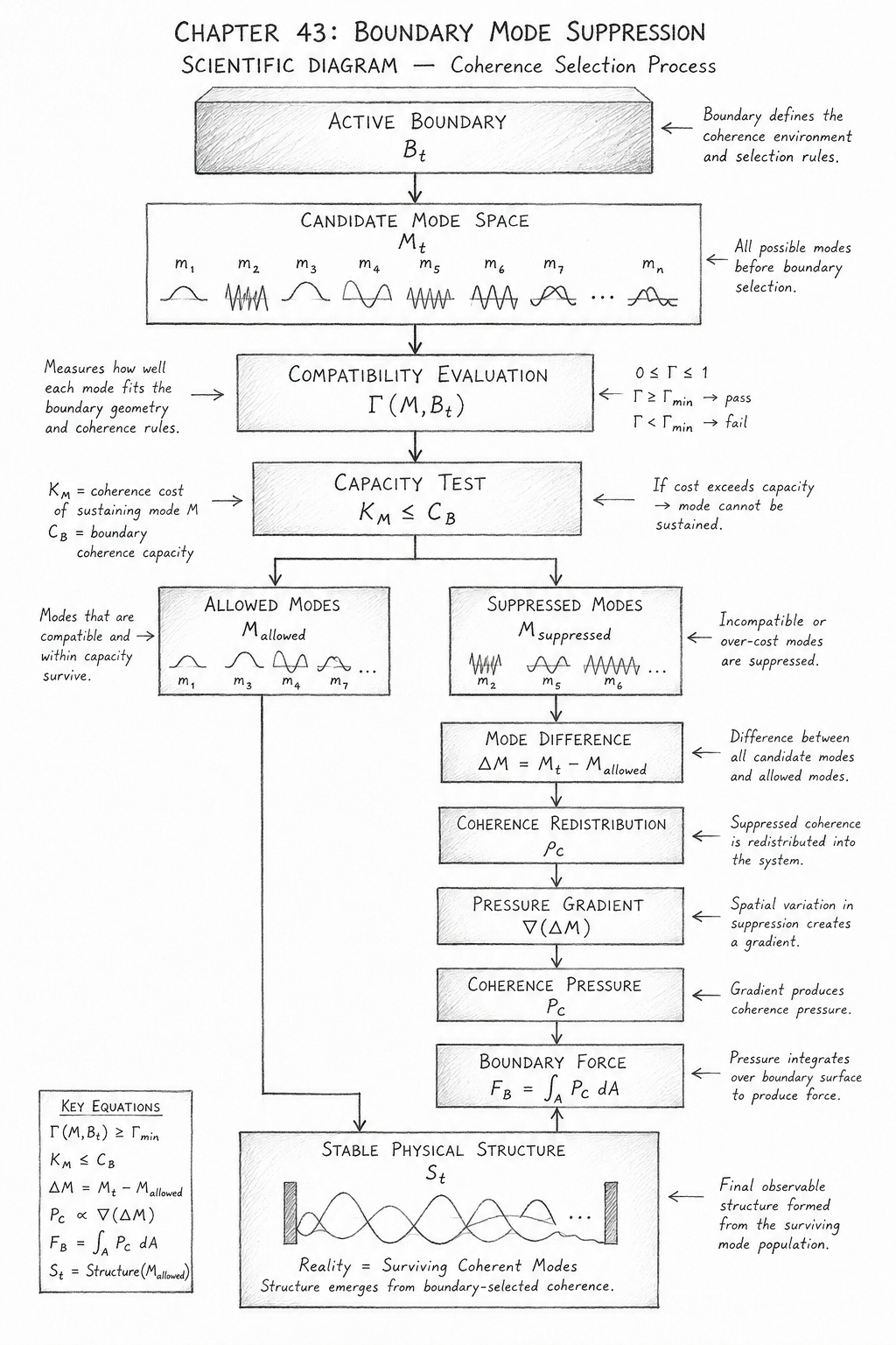
Overview of the Diagram

This diagram illustrates one of the central selection mechanisms within Holographic Space-Time (HST) theory: Boundary Mode Suppression.

The figure demonstrates how a boundary acts as an active coherence filter, determining which field configurations are capable of stable existence and which are removed from the physically realizable state space.

Unlike conventional interpretations that treat boundaries as passive constraints, the HST framework views boundaries as dynamic selection structures that continuously evaluate candidate modes according to coherence compatibility and support capacity.

The complete diagram follows the progression:

\[ B_t \rightarrow M_t \rightarrow \Gamma \left( M, B_t \right) \rightarrow K_M \rightarrow C_B \rightarrow M_{\mathrm{allowed}} \rightarrow M_{\mathrm{suppressed}} \rightarrow \rho_C \rightarrow \nabla \left( \Delta M \right) \rightarrow P_C \rightarrow F_B \rightarrow S_t \]

This sequence represents the transformation of possibility into physical structure.

Active Boundary BtB_t

At the top of the figure sits the active boundary.

\[ B_t \]

The boundary represents the physical or coherence geometry defining the environment in which modes attempt to exist.

Examples include:

  • Conducting plates
  • Optical fibre walls
  • Atomic potentials
  • Crystal boundaries
  • Resonant cavities
  • Material interfaces

Within HST the boundary is not simply a geometric edge.
It is a coherence-selective structure containing information about:

  • Permitted wavelengths
  • Allowed curvatures
  • Supportable phase relationships
  • Information storage capacity

The boundary therefore acts as the governing rule set for all subsequent selection processes.

Candidate Mode Space MtM_t

The second block contains the complete candidate mode population:

\[ M_t \]

represented in the diagram by multiple wave-like structures:

\[ m_1, m_2, m_3, m_4, m_5, m_6, m_7, \ldots \]

Each mode represents a possible field configuration.

Examples include:

  • Standing waves
  • Resonant oscillations
  • Curvature distributions
  • Quantum states
  • Electromagnetic patterns

At this stage the modes are merely possibilities.

No selection has yet occurred.

The diagram intentionally depicts all modes together because the system initially considers every candidate configuration available within the field.

Compatibility Evaluation Γ(M,Bt)\Gamma(M,B_t)

The first major filtering stage is the compatibility evaluation.

\[ \Gamma \left( M, B_t \right) \]

This function measures how effectively a mode aligns with the structural requirements imposed by the boundary.

The diagram notes:

\[ 0 \leq \Gamma \leq 1 \]

where:

  • Γ≈1\Gamma \approx 1 indicates excellent compatibility
  • Γ≈0\Gamma \approx 0 indicates severe incompatibility

The compatibility evaluation assesses:

Geometric Alignment

Does the mode fit the available boundary dimensions?

Phase Alignment

Can the oscillatory structure remain synchronised with surrounding regions?

Curvature Alignment

Can the local geometry support the mode's curvature demands?

Information Alignment

Can the boundary encode the mode without contradiction?

Only sufficiently aligned modes proceed to the next stage.

Capacity Test KM≤CBK_M \leq C_B

After compatibility evaluation, each mode undergoes a capacity assessment.

The diagram introduces:

\[ K_M \]

the coherence cost of maintaining the mode.

This is compared against:

\[ C_B \]

the maximum coherence capacity of the boundary.

The decision rule is:

\[ K_M \leq C_B \]

This stage determines whether the boundary possesses sufficient resources to sustain the configuration.

A mode may fit geometrically but still fail because it requires excessive coherence support.

The capacity test therefore acts as a second selection filter.

Allowed Modes MallowedM_{allowed}

Modes passing both tests enter:

\[ M_{\mathrm{allowed}} \]

The diagram shows examples:

\[ m_1, m_3, m_4, m_7 \]

These surviving modes form the foundation of the observable structure.

They represent configurations that satisfy:

\[ \Gamma \left( M, B_t \right) \geq \Gamma_{\mathrm{min}} \]

and

\[ K_M \leq C_B \]

The allowed-mode block symbolises successful structural adaptation.

These modes become the building blocks of physical reality.

Suppressed Modes MsuppressedM_{suppressed}

Modes failing either selection criterion enter:

\[ M_{\mathrm{suppressed}} \]

The diagram shows examples:

\[ m_2, m_5, m_6 \]

These modes may fail because:

  • Their wavelength does not fit.
  • Their curvature is excessive.
  • Their phase structure conflicts with neighbours.
  • Their coherence cost exceeds available capacity.

Suppression removes these configurations from the physically realizable state space.

Importantly, suppression is not treated as destruction.

The coherence associated with the mode is redistributed throughout the system.

Mode Difference ΔM\Delta M

The next stage computes:

\[ \Delta M = M_t - M_{\mathrm{allowed}} \]

This quantity measures the total amount of suppression occurring within the system.

Physically:

\[ \Delta M \]

represents missing configuration space.

The diagram places this stage immediately beneath the suppressed modes because it quantifies the consequences of their removal.

Coherence Redistribution ρC\rho_C

Suppression alters the surrounding coherence field.

The diagram therefore introduces:

\[ \rho_C \]

representing the redistributed coherence density.

The system responds to missing modes by reorganising available coherence resources.

This redistribution produces:

  • Local density changes
  • Curvature adjustments
  • Stability shifts
  • Pressure imbalances

The diagram highlights this step because it transforms mode suppression into physically measurable consequences.

Pressure Gradient ∇(ΔM)\nabla(\Delta M)

Redistribution produces spatial variation in suppression.

This variation appears as:

\[ \nabla \left( \Delta M \right) \]

The gradient indicates that suppression is not uniformly distributed throughout the system.

Some regions contain larger mode deficits than others.

This imbalance generates directional coherence pressure.

The gradient block therefore marks the transition from structural selection to force generation.

Coherence Pressure PCP_C

The next block represents:

\[ P_C \]

which obeys:

\[ P_C \propto \nabla \left( \Delta M \right) \]

The pressure is not mechanical in the classical sense.

Instead, it reflects the tendency of the coherence field to minimise structural imbalance.

Regions containing stronger suppression gradients generate larger coherence pressures.

The diagram positions this stage immediately before force generation because pressure acts as the intermediary between suppression and observable dynamics.

Boundary Force FBF_B

The pressure accumulates across the boundary surface:

\[ F_B = \int_{A} P_C \, dA \]

This integral converts distributed coherence pressure into a measurable force.

The diagram highlights this stage because it explains how a purely structural selection process can generate observable physical effects.

Within HST, forces emerge naturally from coherence imbalances rather than requiring independent force-generating mechanisms.

Telephone:
01377 236594

Stable Physical Structure StS_t

At the bottom of the figure lies the final result:

\[ S_t \]

The stable structure is constructed exclusively from:

Mallowed​

The surviving coherent modes combine to form the observable physical system.

The diagram shows standing-wave structures inside the final box to illustrate that reality consists of the surviving configurations after selection has occurred.

The caption beneath the structure states:

Reality = Surviving Coherent Modes

This sentence summarises the entire chapter.

Casimir Interpretation of the Diagram

Although the figure is general, it directly explains the Casimir Effect.

In the Casimir case:

\[ M_{\mathrm{inside}} < M_{\mathrm{outside}} \]

The conducting plates suppress internal modes.

This creates:

\[ \Delta M \]

between interior and exterior regions.

The resulting suppression gradient generates:

\[ P_C \]

which integrates into:

\[ F_C \]

the observable Casimir attraction.

Thus the diagram provides a complete HST interpretation of Casimir forces as a consequence of boundary-driven mode suppression.

Scientific Significance of the Diagram

This figure visually unifies several traditionally separate areas of physics:

  • Standing waves
  • Resonance
  • Quantum confinement
  • Atomic orbitals
  • Waveguides
  • Casimir forces
  • Mode selection

The diagram shows that all can be understood through a single process:

  • 1. Define a boundary.
  • 2. Generate candidate modes.
  • 3. Test compatibility.
  • 4. Test capacity.
  • 5. Preserve viable modes.
  • 6. Suppress incompatible modes.
  • 7. Redistribute coherence.
  • 8. Generate gradients.
  • 9. Generate pressure.
  • 10. Generate force.
  • 11. Produce stable structure.

Within HST, physical reality is therefore not viewed as a collection of independently existing objects, but as the surviving residue of an ongoing coherence-selection process governed by boundaries.

The diagram captures this entire mechanism in a single visual framework, making Boundary Mode Suppression one of the foundational organisational principles of the theory.

Diagram → Flow Mapping Table

Diagram Element Flow Symbol Flow Section Scientific Meaning
Active Boundary B_t boundary Defines the coherence environment and selection rules
Boundary Box B_t Input Layer Physical or coherence boundary controlling mode survival
Candidate Mode Space M_t field_modes Complete set of possible field configurations
Individual Modes (m₁,m₂,m₃...) M_t Candidate Population Possible wavelengths, oscillations, or curvature states
Compatibility Evaluation Box Γ(M,B_t) evaluate_modes Measures mode-boundary coherence alignment
Compatibility Threshold Γ_min Preservation Test Minimum compatibility required for survival
Capacity Test Box K_M ≤ C_B capacity_test Determines whether the boundary can support the mode
Coherence Cost Label K_M Cost Computation Structural burden of maintaining a mode
Boundary Capacity Label C_B Capacity Layer Maximum coherence load supportable by boundary
Decision Branch Pass / Fail Selection Logic Separates viable and non-viable configurations
Allowed Modes Box M_allowed preserve_mode Modes surviving compatibility and capacity tests
Surviving Modes (m₁,m₃,m₄,m₇) M_allowed Stable Population Physically realizable configurations
Suppressed Modes Box M_suppressed suppress_mode Modes removed from realizable state space
Rejected Modes (m₂,m₅,m₆) M_suppressed Suppressed Population Incompatible or over-cost configurations
Mode Difference Box ΔM Suppression Layer Total suppressed mode content
Coherence Redistribution Box ρ_C redistribute Reorganisation of coherence after suppression
Pressure Gradient Box ∇(ΔM) Gradient Formation Spatial variation of suppression
Coherence Pressure Box P_C Pressure Generation Pressure arising from suppression imbalance
Boundary Force Box F_B Force Generation Integrated coherence pressure over boundary
Stable Physical Structure Box S_t Output Layer Observable structure formed from surviving modes
Standing Waves in Structure M_allowed Final State Surviving coherent configurations
Reality = Surviving Coherent Modes S_t = Structure(M_allowed) Final Interpretation Physical reality emerges from mode selection

Diagram Path → Flow Path Mapping

Diagram Path Flow Execution
Active Boundary Created B_t
Candidate Modes Generated M_t
Compatibility Measured Γ(M,B_t)
Coherence Cost Computed K_M
Boundary Capacity Evaluated C_B
Capacity Test Applied K_M ≤ C_B
Compatible Modes Preserved M_allowed
Incompatible Modes Suppressed M_suppressed
Mode Deficit Calculated ΔM
Coherence Redistributed ρ_C
Suppression Gradient Formed ∇(ΔM)
Pressure Generated P_C
Force Generated F_B
Stable Structure Produced S_t

Casimir Interpretation Mapping

Diagram Feature Casimir Equivalent HST Meaning
Boundary Box Conducting Plates Mode-selective surfaces
Candidate Modes Vacuum Fluctuation Modes Available coherence configurations
Allowed Modes M_inside Modes fitting between plates
Suppressed Modes Missing Internal Modes Excluded configurations
Mode Difference M_outside - M_inside Suppression imbalance
Pressure Gradient P_C Coherence pressure difference
Boundary Force F_C Casimir attraction
Stable Structure Equilibrium Plate System Minimum contradiction state

Flow Chain ⇔ Equation Chain

Flow Sequence Equation Sequence
Boundary Defined B_t
Candidate Modes Generated M_t
Compatibility Evaluated Γ(M,B_t)
Cost Computed K_M
Capacity Tested K_M ≤ C_B
Allowed Modes Selected M_allowed
Incompatible Modes Removed M_suppressed
Coherence Redistributed ρ_C'
Suppression Gradient Forms ∇(ΔM)
Pressure Generated P_C
Force Generated F_B
Stable Structure Emerges S_t

Complete Diagram Flow Chain

ACTIVE BOUNDARY
      ↓
B_t
      ↓
M_t
      ↓
Γ(M,B_t)
      ↓
K_M ≤ C_B
      ↓
 ┌───────────────┬───────────────┐
 │               │
 ▼               ▼
M_allowed   M_suppressed
 │               │
 │               ▼
 │             ΔM
 │               ▼
 │             ρ_C
 │               ▼
 │           ∇(ΔM)
 │               ▼
 │             P_C
 │               ▼
 │             F_B
 │
 ▼
S_t

Ultra-Compact Scientist Summary

Bt​→Mt​→Γ(M,Bt​)→KM​→CB​→Mallowed​→Msuppressed​→ΔM→ρC​→∇(ΔM)→PC​→FB​→St​

Diagram Interpretation: The boundary continuously evaluates candidate modes, preserves coherence-compatible structures, suppresses incompatible configurations, redistributes coherence, generates pressure gradients, produces forces, and ultimately constructs the stable physical structures observed in reality.

Execution Guarantee Statement

Formal Execution Guarantee

The Boundary Mode Suppression Flow is guaranteed to produce a physically admissible stable structure whenever a boundary exists, candidate modes are present, and at least one mode satisfies both the compatibility and capacity constraints.

Formally:

\[ \exists M_i \in M_t \]

such that

\[ \Gamma \left( M_i, B_t \right) \geq \Gamma_{\mathrm{min}} \]

and

\[ K_M \left( M_i \right) \leq C_B \]

implies

\[ M_{\mathrm{allowed}} \neq \emptyset \]

which guarantees

Therefore:

\[ M_{\mathrm{allowed}} \neq \emptyset \Rightarrow \mathrm{Execution} \left( S_t \right) = \mathrm{SUCCESS} \]

Boundary Selection Guarantee

The flow guarantees that no mode may enter the final structure without passing both selection tests.

Every surviving mode must satisfy:

\[ \Gamma \left( M, B_t \right) \geq \Gamma_{\mathrm{min}} \]

and

\[ K_M \leq C_B \]

Therefore:

\[ M_{\mathrm{allowed}} = \left\{ M \in M_t \;\middle|\; \Gamma \left( M, B_t \right) \geq \Gamma_{\mathrm{min}} \;\land\; K_M \leq C_B \right\} \]

No incompatible mode can survive.

No compatible mode is removed unnecessarily.

The selection process is deterministic.

Suppression Guarantee

The flow guarantees that every rejected mode possesses a measurable cause for suppression.

A mode enters

Msuppressed​

if and only if:

\[ \Gamma \left( M, B_t \right) < \Gamma_{\mathrm{min}} \]

or

\[ K_M > C_B \]

Thus:

\[ M_{\mathrm{suppressed}} = \left\{ M \in M_t \;\middle|\; \Gamma \left( M, B_t \right) < \Gamma_{\mathrm{min}} \;\lor\; K_M > C_B \right\} \]

Suppression is never arbitrary.

Every rejection results from explicit boundary incompatibility or capacity overload.

Coherence Conservation Guarantee

The flow guarantees that suppression does not destroy coherence information.

Instead:

\[ M_{\mathrm{suppressed}} \rightarrow \Delta \rho_C \]

leading to

\[ \rho_C' = \rho_C + \Delta \rho_C \]

Suppressed coherence is redistributed throughout the surrounding system.

Therefore:

Informationtotal​=Constant

within the model.

The flow preserves coherence accounting at every stage.

Pressure Formation Guarantee

Whenever suppression is spatially non-uniform:

\[ \nabla \left( \Delta M \right) \neq 0 \]

the flow guarantees emergence of coherence pressure:

\[ P_C \propto \nabla \left( \Delta M \right) \]

Thus:

\[ \nabla \left( \Delta M \right) \neq 0 \Rightarrow P_C > 0 \]

Pressure generation is therefore an inevitable consequence of suppression imbalance.

Force Generation Guarantee

Whenever coherence pressure exists across a finite boundary area:

\[ P_C > 0 \]

the flow guarantees force generation:

\[ F_B = \int_{A} P_C \, dA \]

Therefore:

\[ P_C > 0 \Rightarrow F_B > 0 \]

Observable forces emerge automatically from suppression-driven pressure gradients.

Structural Stability Guarantee

The final structure:

\[ S_t = \mathrm{Structure} \left( M_{\mathrm{allowed}} \right) \]

is guaranteed to contain only modes capable of satisfying both compatibility and capacity requirements.

Thus:

\[ \forall M_i \in S_t \]

\[ \Gamma \left( M_i, B_t \right) \geq \Gamma_{\mathrm{min}} \]

and

\[ K_M \left( M_i \right) \leq C_B \]

The resulting structure is therefore internally self-consistent relative to its boundary.

Casimir Guarantee

For the special case:

\[ M_{\mathrm{inside}} < M_{\mathrm{outside}} \]

the flow guarantees:

\[ \Delta M > 0 \]

which guarantees:

\[ P_C > 0 \]

which guarantees:

\[ F_C > 0 \]

Thus:

\[ M_{\mathrm{inside}} < M_{\mathrm{outside}} \Rightarrow F_C > 0 \]

The Casimir force emerges automatically from boundary mode suppression.

Failure Guarantee

The flow will terminate in failure only if:

No Compatible Modes Exist

\[ \forall M_i \in M_t \]

\[ \Gamma \left( M_i, B_t \right) < \Gamma_{\mathrm{min}} \]

or

Boundary Capacity Is Exceeded

\[ K_M > C_B \]

for every candidate mode.

Result:

\[ M_{\mathrm{allowed}} = \emptyset \]

and therefore:

\[ S_t = \emptyset \]

yielding

\[ \mathrm{Execution} = \mathrm{FAIL} \]

Complete Execution Guarantee

Bt​→Mt​→Γ(M,Bt​)→KM​→CB​→Mallowed​→Msuppressed​→ΔM→ρC​→∇(ΔM)→PC​→FB​→St​

Guaranteed Outcome

If a boundary exists and at least one candidate mode satisfies the minimum compatibility requirement and the boundary capacity constraint, the flow will deterministically construct a stable physical structure from the surviving mode population, redistribute suppressed coherence, generate any resulting pressure gradients and forces, and converge to a boundary-consistent final state.

\[ \exists M_i : \Gamma \left( M_i, B_t \right) \geq \Gamma_{\mathrm{min}} \;\land\; K_M \left( M_i \right) \leq C_B \]

⟹

\[ \mathrm{Execution} \left( S_t \right) = \mathrm{GUARANTEED} \]

HST Interpretation: Reality emerges through boundary-driven selection. Any mode compatible with the boundary survives, any incompatible mode is suppressed, coherence is conserved through redistribution, and stable structure inevitably forms from the surviving coherent population.

Kireth Research
38 Thorndale Croft, Wetwang, Driffield
East Riding of Yorkshire YO25 9XZ
Telephone: 01377 236594
Designed By