Chapter 42
Fibre Optics and Transparent Geometry

Photons and Coherence Geometry
Author: Mark Higgins
© Mark Anthony Higgins 11 October 2025
Revised Date: 17 June 2026
Audio Overview

Introduction

Fibre optics is often presented as one of the clearest demonstrations of light bending through space. In conventional physics, photons are described as continuously refracting within a material due to changes in refractive index, producing smooth curved trajectories that guide light through optical fibres.

Within the Holographic Space-Time (HST) framework, however, fibre optics provides a powerful example of a deeper principle: the distinction between actual propagation and observed interpretation.

HST proposes that photons do not physically travel along continuously curved paths. Instead, they propagate through a sequence of locally coherent transfers across boundary structures. What appears to observers as a curved trajectory emerges from the accumulation of many small alignment events occurring within the optical medium. The apparent curve is therefore a geometric interpretation generated by boundary coherence rather than a literal bending of the photon's path.

This chapter extends the concepts developed in previous discussions of wave propagation, photon geometry, and flat-path transport. It demonstrates how optical fibres can be understood as coherence-guiding structures that continuously realign photon propagation without requiring the existence of intrinsically curved motion.

42.1 The Conventional Interpretation of Fibre Optics

In standard electromagnetic theory, light entering a fibre experiences repeated refraction caused by differences in refractive index between the fibre core and cladding.

The classical picture states:

  • Photons enter the fibre.
  • Electromagnetic waves interact with the material.
  • Refraction redirects propagation.
  • Internal reflection confines the light.
  • Curved fibres bend the light path.

From this viewpoint, the photon trajectory itself is considered curved.

The observed output of the fibre is entirely consistent with this interpretation and accurately predicts engineering behaviour.

However, HST asks a deeper question:

Does the photon actually travel along a curved path, or is curvature merely the accumulated appearance of many locally flat transfers?

42.2 Local Flatness Inside the Fibre

HST begins from a fundamental geometric principle:

Propagation occurs through local coherence alignment.

A photon does not move by following a pre-existing curved trajectory.

Instead:

  • 1. Local boundary structure is encountered.
  • 2. Coherence gradients are evaluated.
  • 3. Propagation aligns with the strongest coherent direction.
  • 5. A small transfer occurs.
  • 6. The process repeats.

At each microscopic step the propagation remains locally straight.

Symbolically:

\[ \mathrm{Path}_{\mathrm{local}} \approx \mathrm{Straight} \]

No individual transfer requires curvature.

Only after many sequential transfers do observers reconstruct a larger trajectory.

42.3 Optical Fibres as Coherence Guides

Within HST, an optical fibre acts as a structured coherence channel.

The fibre geometry continuously shapes the available coherence landscape.

As photons propagate:

\[ B_t \rightarrow C_t \]

where:

  • BtB_t represents local boundary structure.
  • CtC_t represents the coherence map generated by that structure.

The photon then aligns with:

\[ \nabla \rho_C \]

the local coherence gradient.

This process repeats thousands or millions of times along the fibre.

The fibre therefore acts not as a curved tunnel through which photons physically bend, but as a coherence-guidance system that repeatedly updates propagation direction.

42.4 Apparent Curvature from Sequential Alignment

Consider a gently curved optical fibre.

At any microscopic location:

  • The fibre wall defines local boundary conditions.
  • Coherence gradients shift slightly.
  • Propagation realigns.
  • A new local straight segment is executed.

The resulting motion resembles:

\[ \mathrm{Path}_{\mathrm{global}} = \sum \mathrm{Path}_{\mathrm{local}} \]

where every local component remains approximately flat.

Observers reconstruct:

\[ \mathrm{Path}_{\mathrm{global}} \approx \mathrm{Curved} \]

even though no individual propagation event requires continuous curvature.

This is analogous to approximating a circle using an enormous number of tiny straight-line segments.

The circle appears smooth despite being constructed from locally flat components.

42.5 Transparent Geometry

Transparent materials provide a particularly important example of HST geometry.

In conventional theory, transparency is often treated as a consequence of quantum interactions that do not absorb visible photons.

HST extends this interpretation.

A transparent medium is a material whose boundary structure allows coherence transfer with minimal disruption.

Formally:

\[ \mathrm{Disruption}(C_t) \rightarrow \mathrm{Min} \]

When disruption remains low:

\[ \mathrm{Propagation} \rightarrow \mathrm{Stable} \]

and photons continue transferring through the medium.

Transparency therefore emerges when boundary geometry preserves coherence continuity rather than destroying it.

42.6 Why Light Appears to Bend

A key prediction of HST is that observed bending is often a reconstruction effect.

Observers measure:

  • Entry position.
  • Exit position.
  • Transit time.

A trajectory is then inferred.

However, the inferred curve is not necessarily the actual propagation geometry.

Instead:

Observed Curvature=Interpretation(Local Transfers)

This principle has already appeared in:

  • Field line formation
  • Gradient flow
  • Wave propagation
  • Photon trajectories

Fibre optics provides another example where the distinction becomes visible.

42.7 Relationship to Photons and Coherence Geometry

Chapter 41 demonstrated that photons travel through locally flat coherence transfers.

This chapter extends that framework into real optical systems.

The progression becomes:

  • 1. Boundary structure exists.
  • 2. Coherence map forms.
  • 3. Gradients emerge.
  • 4. Propagation aligns locally.
  • 5. Transfer occurs.
  • 6. Alignment updates.
  • 7. Apparent curvature accumulates.

Symbolically:

\[ B_t \rightarrow C_t \rightarrow \rho_C \rightarrow \nabla \rho_C \rightarrow R_t \rightarrow x_{t+1} \]

Repeated execution produces the observable optical path.

Thus fibre optics becomes a practical engineering manifestation of the broader HST principle that:

Global curvature can emerge from sequences of locally flat coherence transfers.

42.8 Scientific Significance

The HST interpretation does not alter the successful engineering predictions of fibre optic theory.

Optical communication systems continue to function exactly as observed.

What changes is the geometric interpretation of propagation.

Instead of assuming:

\[ \mathrm{Photon} \rightarrow \mathrm{Curved\ Path} \]

HST proposes:

\[ \mathrm{Photon} \rightarrow \mathrm{Local\ Coherence\ Transfers} \rightarrow \mathrm{Apparent\ Curvature} \]

This shifts the explanatory foundation from continuous path bending to recursive boundary-guided alignment.

The result is a unified description connecting:

  • Fibre optics
  • Refraction
  • Wave propagation
  • Electromagnetic fields
  • Curvature interpretation
  • Photon transport

under a single coherence-based geometric framework.


Conclusion

Fibre optics provides one of the clearest physical demonstrations of how apparent curvature can emerge from locally flat propagation. Within HST, optical fibres are interpreted as coherence-guidance structures that continuously realign photon transfer through evolving boundary conditions.

The photon does not require a fundamentally curved trajectory. Instead, curvature emerges as the large-scale interpretation of countless microscopic alignment events.

Transparent geometry therefore becomes a direct manifestation of boundary coherence, reinforcing the broader HST principle that observed motion, fields, and curvature arise from recursive local interactions rather than pre-existing geometric distortions of space itself.

Flow: FibreOptics_TransparentGeometry
Version: 1.0
Authors:
  - Mark Higgins
  - Sky Recursive AI

Purpose:
  To model fibre optics as boundary-guided coherent propagation,
  where globally curved light paths emerge from sequences of locally
  flat photon-transfer updates through transparent geometry.

Domain:
  Theory: HST
  Chapter: 42
  Topic: Fibre Optics and Transparent Geometry

Inputs:
  B_t:
    description: Local fibre boundary state at time t
    type: boundary_geometry

  n_core:
    description: Refractive coherence density of fibre core
    type: scalar_field

  n_cladding:
    description: Refractive coherence density of surrounding cladding
    type: scalar_field

  P_t:
    description: Photon propagation state at time t
    type: propagation_state

  x_t:
    description: Photon position at time t
    type: spatial_state

  theta_t:
    description: Local propagation angle
    type: angular_state

Parameters:
  C_min:
    description: Minimum coherence required for stable propagation
    type: threshold

  G_max:
    description: Maximum permitted coherence-gradient discontinuity
    type: threshold

  theta_crit:
    description: Critical confinement angle for guided propagation
    type: angle_threshold

  epsilon_flat:
    description: Maximum permitted curvature of each local segment
    type: tolerance

  c_limit:
    description: Maximum allowed propagation speed
    type: causal_limit

Derived_States:
  C_t:
    expression: CoherenceMap(B_t, n_core, n_cladding)
    meaning: Local coherence map generated by fibre boundary geometry

  rho_C:
    expression: Density(C_t)
    meaning: Coherence-density landscape inside the fibre

  grad_rho_C:
    expression: Gradient(rho_C)
    meaning: Local directional coherence gradient

  Delta_n:
    expression: n_core - n_cladding
    meaning: Coherence contrast between core and cladding

  R_t:
    expression: Align(P_t, grad_rho_C)
    meaning: Local propagation realignment vector

  theta_t_next:
    expression: UpdateAngle(theta_t, R_t)
    meaning: Updated local propagation angle after boundary alignment

  x_t_next:
    expression: x_t + LocalStep(R_t)
    meaning: Next photon position after locally flat transfer

  Path_local:
    expression: Segment(x_t, x_t_next)
    meaning: Individual locally flat propagation segment

  Path_global:
    expression: Sum(Path_local)
    meaning: Reconstructed large-scale fibre trajectory

  K_app:
    expression: Curvature(Path_global)
    meaning: Apparent curvature inferred by external observation

Process:
  Step_1_Boundary_Encoding:
    input: B_t
    output: C_t
    operation: CoherenceMap(B_t, n_core, n_cladding)
    meaning: Fibre geometry encodes a local coherence field.

  Step_2_Coherence_Density:
    input: C_t
    output: rho_C
    operation: Density(C_t)
    meaning: Coherence density defines where transparent transfer remains stable.

  Step_3_Gradient_Formation:
    input: rho_C
    output: grad_rho_C
    operation: Gradient(rho_C)
    meaning: Directional coherence gradients guide photon transfer.

  Step_4_Core_Cladding_Contrast:
    input:
      - n_core
      - n_cladding
    output: Delta_n
    operation: n_core - n_cladding
    meaning: Coherence contrast creates confinement between fibre core and cladding.

  Step_5_Local_Realignment:
    input:
      - P_t
      - grad_rho_C
    output: R_t
    operation: Align(P_t, grad_rho_C)
    meaning: Photon propagation aligns with the strongest locally coherent direction.

  Step_6_Angle_Update:
    input:
      - theta_t
      - R_t
    output: theta_t_next
    operation: UpdateAngle(theta_t, R_t)
    meaning: The local propagation angle updates without requiring global path curvature.

  Step_7_Local_Transfer:
    input:
      - x_t
      - R_t
    output: x_t_next
    operation: x_t + LocalStep(R_t)
    meaning: Photon state advances by one locally flat transfer.

  Step_8_Local_Path_Record:
    input:
      - x_t
      - x_t_next
    output: Path_local
    operation: Segment(x_t, x_t_next)
    meaning: Each microscopic transfer remains approximately straight.

  Step_9_Global_Path_Reconstruction:
    input: Path_local
    output: Path_global
    operation: Sum(Path_local)
    meaning: Many local flat transfers accumulate into an observed fibre path.

  Step_10_Apparent_Curvature:
    input: Path_global
    output: K_app
    operation: Curvature(Path_global)
    meaning: Curvature is reconstructed from accumulated alignment updates.

Invariants:
  Local_Flatness:
    expression: Curvature(Path_local) <= epsilon_flat
    meaning: Each local photon-transfer segment remains approximately flat.

  Coherence_Continuity:
    expression: C_t >= C_min
    meaning: Propagation continues only if coherence remains above threshold.

  Gradient_Smoothness:
    expression: Discontinuity(grad_rho_C) <= G_max
    meaning: Coherence gradients must change smoothly enough for stable transfer.

  Core_Confinement:
    expression: Delta_n > 0
    meaning: Fibre core must maintain higher guiding coherence than cladding.

  Critical_Angle_Condition:
    expression: theta_t <= theta_crit
    meaning: Photon propagation remains confined within the fibre guidance channel.

  Causal_Limit:
    expression: Velocity(P_t) <= c_limit
    meaning: Propagation cannot exceed the causal speed limit.

Failure_States:
  Coherence_Collapse:
    condition: C_t < C_min
    result: Propagation becomes unstable or terminates.

  Gradient_Discontinuity:
    condition: Discontinuity(grad_rho_C) > G_max
    result: Photon transfer scatters, leaks, or decoheres.

  Confinement_Failure:
    condition: Delta_n <= 0
    result: Fibre no longer provides stable guidance.

  Critical_Angle_Exceeded:
    condition: theta_t > theta_crit
    result: Photon escapes the core guidance channel.

  Local_Curvature_Failure:
    condition: Curvature(Path_local) > epsilon_flat
    result: Local transfer violates flat-path propagation.

  Causal_Violation:
    condition: Velocity(P_t) > c_limit
    result: Execution(P_t) = FAIL

Execution:
  Initial_State:
    input:
      - B_t
      - n_core
      - n_cladding
      - P_t
      - x_t
      - theta_t

  Recursive_Update:
    chain:
      - B_t
      - C_t
      - rho_C
      - grad_rho_C
      - Delta_n
      - R_t
      - theta_t_next
      - x_t_next
      - Path_local
      - Path_global
      - K_app

  Success_Condition:
    expression: >
      C_t >= C_min
      and Discontinuity(grad_rho_C) <= G_max
      and Delta_n > 0
      and theta_t <= theta_crit
      and Curvature(Path_local) <= epsilon_flat
      and Velocity(P_t) <= c_limit

  Output:
    if Success_Condition:
      Execution(P_t): GUIDED_PROPAGATION
      Interpretation: Apparent global curvature from locally flat coherent transfers

    else:
      Execution(P_t): FAIL_OR_LEAK
      Interpretation: Fibre guidance breaks through decoherence, scattering, leakage, or causal violation

Scientific_Claim:
  Statement: >
    Fibre optics does not require photons to travel along intrinsically
    curved paths. Within HST, optical fibres operate as transparent
    coherence-guidance structures, where each photon transfer is locally
    flat and globally reconstructed as curved through repeated boundary
    alignment.

Compact_Equation_Form:
  Boundary_To_Curvature:
    expression: B_t -> C_t -> rho_C -> grad_rho_C -> R_t -> x_t_next -> Path_global -> K_app

  Local_Flat_Global_Curved:
    expression: Sum(Path_local_flat) -> Path_global_curved

  Transparent_Guidance:
    expression: C_t >= C_min and Delta_n > 0 -> Execution(P_t) = GUIDED_PROPAGATION

What This Flow Implements

Overview

This flow implements an HST-based reformulation of fibre optic propagation in which light transmission is interpreted as a sequence of coherent boundary-guided transfer events rather than the motion of photons along intrinsically curved trajectories.

The flow models an optical fibre as a structured coherence-guidance system. The fibre core, cladding, and internal material geometry generate coherence gradients that continuously realign photon propagation. Each propagation step remains locally flat, while the accumulation of many such transfers produces the appearance of a globally curved path.

The central claim implemented by the flow is:

Apparent optical curvature emerges from recursive local coherence alignment rather than continuous path bending.

The flow therefore provides a complete execution model for fibre-optic transport within the Holographic Space-Time framework.

Fibre Optics as Boundary-Guided Propagation

In conventional electromagnetic theory, fibre optics are explained through refraction and total internal reflection.

The standard interpretation assumes that light continuously bends as it travels through the fibre.

This flow implements an alternative geometric description.

Instead of treating curvature as a property of the photon's path, the system models propagation as:

\[ B_t \rightarrow C_t \rightarrow \rho_C \rightarrow \nabla \rho_C \rightarrow R_t \rightarrow x_{t+1} \]

where each propagation update is determined by local coherence structure.

The photon does not require knowledge of the global fibre shape.

Only local coherence conditions influence the next transfer event.

Boundary Geometry Reconstruction

The first component implemented by the flow is boundary encoding.

The fibre structure acts as a boundary system:

\[ B_t \]

containing information about:

  • Core geometry
  • Cladding geometry
  • Material structure
  • Local refractive characteristics
  • Surface conditions

The flow converts this boundary information into a coherence map:

\[ C_t = \mathrm{CoherenceMap}(B_t) \]

This operation creates the internal guidance landscape through which propagation occurs.

Rather than treating the optical fibre as empty space containing a curved light beam, the flow models the fibre itself as an active geometric participant in propagation.

Coherence Density Formation

After boundary reconstruction, the flow generates a coherence density field:

\[ \rho_C = \mathrm{Density}(C_t) \]

This density field represents the local stability of propagation.

Regions of higher coherence density support stable transfer.

Regions of lower coherence density create instability, leakage, or scattering.

The resulting density landscape becomes the effective navigation field for photon transport.

Within HST, this replaces the conventional notion of refractive-index-driven path bending.

Gradient-Based Guidance

The flow next computes:

\[ \nabla \rho_C \]

which represents the local coherence gradient.

This gradient determines the direction of maximum propagation stability.

The photon state:

\[ P_t \]

is aligned with the gradient through:

\[ R_t = \mathrm{Align} \!\left( P_t,\, \nabla \rho_C \right) \]

This operation is one of the most important components of the entire model.

The photon does not "follow a curve."

Instead, it repeatedly chooses the locally optimal coherent direction.

The observed trajectory emerges from these recursive updates.

Core–Cladding Confinement Mechanism

The flow explicitly models the coherence contrast between fibre core and cladding:

\[ \Delta n = n_{\mathrm{core}} - n_{\mathrm{cladding}} \]

This contrast acts as the confinement mechanism.

The condition:

\[ \Delta n > 0 \]

ensures that the fibre core remains the most coherent propagation channel.

As long as this condition is maintained, propagation remains trapped within the fibre.

This reproduces the engineering behaviour of optical fibres while providing a coherence-based explanation.

Local Flat Transfer Execution

A central feature of the flow is the implementation of locally flat propagation.

Each update executes:

\[ x_{t+1} = x_t + \mathrm{LocalStep} \!\left( R_t \right) \]

The resulting path segment is:

Pathlocal​

The flow imposes the invariant:

\[ \mathrm{Curvature} \!\left( \mathrm{Path}_{\mathrm{local}} \right) \leq \epsilon_{\mathrm{flat}} \]

meaning that every individual transfer remains approximately straight.

No microscopic propagation step requires continuous curvature.

This is one of the defining principles of HST geometry.

Emergence of Global Curvature

The flow then accumulates all local transfers:

\[ \mathrm{Path}_{\mathrm{global}} = \sum \mathrm{Path}_{\mathrm{local}} \]

The resulting reconstructed path exhibits:

\[ \kappa = \mathrm{Curvature} \!\left( \mathrm{Path}_{\mathrm{global}} \right) \]

where:

\[ \kappa > 0 \]

may occur despite each individual segment remaining flat.

This section of the flow implements one of the key geometric claims of HST:

Global curvature can emerge from the accumulation of locally flat coherence-guided transfers.

The fibre therefore appears curved even though propagation itself never requires a fundamentally curved path.

Transparent Geometry

The flow also implements the HST concept of transparent geometry.

Transparency is treated as a coherence-preservation phenomenon.

Stable propagation requires:

\[ C_t \geq C_{\min} \]

and

\[ \mathrm{Discontinuity} \!\left( \nabla \rho_C \right) \leq G_{\max} \]

When these conditions hold:

  • Coherence remains continuous.
  • Transfer remains stable.
  • Scattering is minimised.
  • Optical transmission persists.

Transparency therefore emerges as successful coherence transport through boundary structure.

Stability Monitoring

The flow continuously monitors several physical constraints.

These include:

Coherence Continuity

\[ C_t \geq C_{\min} \]

ensuring that sufficient coherence exists for propagation.

Gradient Smoothness

\[ \mathrm{Discontinuity} \!\left( \nabla \rho_C \right) \leq G_{\max} \]

preventing disruptive coherence jumps.

Fibre Confinement

\[ \Delta n > 0 \]

maintaining core guidance.

Critical Angle Stability

\[ \theta_t \leq \theta_{\mathrm{crit}} \]

preventing loss of confinement.

Local Flatness

\[ \mathrm{Curvature} \!\left( \mathrm{Path}_{\mathrm{local}} \right) \leq \epsilon_{\mathrm{flat}} \]

maintaining the HST propagation principle.

Causality

\[ \mathrm{Velocity}(P_t) \leq c \]

ensuring physically valid execution.

These invariants guarantee stable fibre operation.

Failure Mode Implementation

The flow also specifies the conditions under which optical guidance fails.

Failure can occur through:

Coherence Collapse

\[ C_t < C_{\min} \]

Gradient Breakdown

\[ \mathrm{Discontinuity} \!\left( \nabla \rho_C \right) > G_{\max} \]

Loss of Core Guidance

\[ \Delta n \leq 0 \]

Critical Angle Violation

\[ \theta_t > \theta_{\mathrm{crit}} \]

Local Curvature Failure

\[ \mathrm{Curvature} \!\left( \mathrm{Path}_{\mathrm{local}} \right) > \epsilon_{\mathrm{flat}} \]

Causal Violation

\[ \mathrm{Velocity}(P_t) > c \]

When these conditions occur, propagation becomes unstable and execution terminates.

Telephone:
01377 236594

Scientific Significance

This flow provides a complete HST execution model for fibre-optic transport.

Rather than interpreting optical fibres as structures that physically bend photon trajectories, the model interprets them as coherence-guidance systems that repeatedly realign locally flat propagation events.

The flow unifies:

  • Fibre optics
  • Refraction
  • Internal reflection
  • Transparency
  • Photon transport
  • Coherence geometry
  • Apparent curvature

within a single recursive framework.

Most importantly, it implements the HST principle that:

\[ \mathrm{Path}_{\mathrm{local}} \approx \mathrm{Flat} \]

while

\[ \mathrm{Path}_{\mathrm{global}} \approx \mathrm{Curved} \]

demonstrating how complex optical trajectories can emerge from sequences of locally coherent boundary-guided transfers without requiring intrinsically curved motion.

How to Read This Flow

Introduction

This flow describes how optical fibre propagation is represented within the Holographic Space-Time (HST) framework. Unlike conventional fibre-optic theory, which treats light as continuously bending through a medium, this flow models photon transport as a sequence of locally coherent transfer events guided by boundary structure.

To read the flow correctly, it is important to understand that every block represents a physical transformation of information rather than a mathematical shortcut.

The flow should therefore be interpreted as a causal chain of geometric reconstruction:

\[ B_t \rightarrow C_t \rightarrow \rho_C \rightarrow \nabla \rho_C \rightarrow R_t \rightarrow x_{t+1} \rightarrow \mathrm{Path}_{\mathrm{global}} \rightarrow \kappa \]

Each stage generates the conditions required for the next stage.

The flow is read from top to bottom and from left to right.

Step 1 — Read the Boundary State

The flow begins with:

\[ B_t \]

This represents the local fibre boundary configuration at time tt.

It contains information about:

  • Fibre core geometry
  • Cladding geometry
  • Material structure
  • Internal interfaces
  • Local optical conditions

In HST, boundaries are fundamental because they encode the information available to the system.

Nothing propagates until a boundary state exists.

When reading the flow, think of BtB_t as the complete optical environment surrounding the photon at a particular moment.

Step 2 — Construct the Coherence Map

The next operation is:

\[ C_t = \mathrm{CoherenceMap}(B_t) \]

This converts the boundary description into a coherence field.

The coherence map is not the photon itself.

Instead, it is the geometric landscape through which propagation will occur.

The map determines:

  • Stability regions
  • Transfer pathways
  • Confinement zones
  • Propagation opportunities

When reading the flow, imagine this stage as building the navigational terrain that the photon will experience.

Step 3 — Generate the Coherence Density Field

The flow then computes:

\[ \rho_C = \mathrm{Density}(C_t) \]

This produces a measurable coherence density distribution.

The density field identifies where propagation is most stable.

High-density regions correspond to strong coherent support.

Low-density regions correspond to instability.

When reading this section, imagine a topographical map where peaks represent highly coherent regions and valleys represent weak coherence regions.

The photon will naturally favour the most stable regions.

Step 4 — Calculate the Coherence Gradient

The next stage computes:

\[ \nabla \rho_C \]

This is one of the most important steps in the entire flow.

The gradient determines:

  • Direction of maximum coherence increase
  • Local propagation preference
  • Alignment direction

This stage creates the guidance information used by the photon.

When reading the flow, view the gradient as a collection of directional arrows embedded within the coherence field.

These arrows indicate where stable propagation is most likely to occur.

Step 5 — Align Photon Propagation

The flow now evaluates:

\[ R_t = \mathrm{Align} \left( P_t, \nabla \rho_C \right) \]

where:

\[ P_t \]

represents the current photon state.

The alignment operation produces:

\[ R_t \]

which becomes the local propagation vector.

This step is critical.

The photon does not calculate a complete path through the fibre.

Instead, it only determines the next coherent direction.

When reading the flow, think of this as a local steering process rather than global route planning.

Step 6 — Update the Propagation Angle

The flow next performs:

\[ \theta_{t+1} = \mathrm{UpdateAngle} \left( \theta_t, R_t \right) \]

This updates the local propagation angle.

The angle changes because the coherence landscape changes.

Importantly, the flow does not generate curvature directly.

Only a small directional adjustment occurs.

When reading this section, imagine tiny microscopic corrections being applied at every transfer step.

Step 7 — Execute a Local Transfer

The next operation is:

\[ x_{t+1} = x_t + \mathrm{LocalStep} \left( R_t \right) \]

This represents the actual propagation event.

The photon advances one locally coherent step.

The flow defines:

\[ \mathrm{Path}_{\mathrm{local}} = \mathrm{Segment} \left( x_t, x_{t+1} \right) \]

This segment represents the fundamental unit of propagation.

The most important invariant is:

\[ \mathrm{Curvature} \left( \mathrm{Path}_{\mathrm{local}} \right) \leq \epsilon_{\mathrm{flat}} \]

which means the segment remains approximately straight.

When reading the flow, treat every transfer as locally flat.

No microscopic curvature is introduced.

Step 8 — Accumulate Local Segments

After many updates, the flow accumulates:

\[ \mathrm{Path}_{\mathrm{global}} = \sum \mathrm{Path}_{\mathrm{local}} \]

This stage combines all locally flat segments into a larger trajectory.

The accumulation process is where apparent curvature begins to emerge.

When reading the flow, imagine constructing a large curve from thousands of tiny straight segments.

Each segment is flat.

The overall path appears curved.

Step 9 — Measure Apparent Curvature

The flow then computes:

\[ K_{\mathrm{app}} = \mathrm{Curvature} \left( \mathrm{Path}_{\mathrm{global}} \right) \]

This quantity represents the curvature observed by an external observer.

Notice an important distinction:

The flow never calculates curvature at the local transfer level.

Curvature only appears after the complete trajectory has been reconstructed.

When reading this stage, remember:

\[ \mathrm{Path}_{\mathrm{local}} \approx \mathrm{Flat} \]

while

\[ \mathrm{Path}_{\mathrm{global}} \approx \mathrm{Curved} \]

This is one of the central principles of HST geometry.

Step 10 — Evaluate Stability Conditions

Throughout execution, the flow continuously checks its invariants.

These include:

Coherence Stability

\[ C_t \geq C_{\mathrm{min}} \]

Gradient Continuity

\[ \mathrm{Discontinuity} \left( \nabla \rho_C \right) \leq G_{\mathrm{max}} \]

Fibre Confinement

\[ \Delta n > 0 \]

Critical Angle Preservation

\[ \theta_t \leq \theta_{\mathrm{crit}} \]

Local Flatness

Curvature(Pathlocal​)≤ϵflat​

Causality

\[ \mathrm{Velocity} \left( P_t \right) \leq c \]

When reading the flow, these conditions should be viewed as execution requirements.

Propagation remains stable only while all conditions are satisfied.

Understanding the Failure States

The flow also defines conditions that terminate propagation.

Examples include:

\[ C_t < C_{\mathrm{min}} \]

or

\[ \Delta n \leq 0 \]

or

\[ \theta_t > \theta_{\mathrm{crit}} \]

When any failure condition occurs, stable guidance can no longer be maintained.

The flow then transitions to:

\[ \mathrm{Execution} \left( P_t \right) = \mathrm{FAIL} \]

This represents leakage, scattering, decoherence, or loss of confinement.

Reading the Complete Execution Chain

The entire flow can be understood as a recursive coherence-guidance loop:

\[ B_t \rightarrow C_t \rightarrow \rho_C \rightarrow \nabla \rho_C \rightarrow R_t \rightarrow \theta_{t+1} \rightarrow x_{t+1} \rightarrow \mathrm{Path}_{\mathrm{local}} \rightarrow \mathrm{Path}_{\mathrm{global}} \rightarrow K_{\mathrm{app}} \]

Read this chain as:

Boundary structure creates coherence.
↓
Coherence creates density.
↓
Density creates gradients.
↓
Gradients guide propagation.
↓
Propagation generates local transfers.
↓
Local transfers accumulate into global trajectories.
↓
Global trajectories create the appearance of curvature.

Scientific Interpretation

The purpose of this flow is not simply to describe fibre optics.

Its deeper role is to demonstrate one of the central geometric principles of HST:

Apparent curvature does not require fundamentally curved propagation.

Instead:

\[ \mathrm{Local\ Transfers} \rightarrow \mathrm{Flat} \]

while

\[ \mathrm{Accumulated\ Transfers} \rightarrow \mathrm{Curved} \]

Thus, when reading this flow, interpret the optical fibre not as a device that bends photons, but as a structured coherence-guidance system that continuously realigns locally flat propagation events.

The observed curved optical path emerges only after these individual transfers are accumulated and reconstructed at larger scales.

Flow → Equation Tri-Mapping Table

Flow Layer Equation Layer Scientific Interpretation
Fibre Boundary State B_t Local optical fibre geometry and material structure
Core–Cladding Encoding n_core, n_cladding Optical coherence densities defining the guidance channel
Coherence Reconstruction C_t = CoherenceMap(B_t,n_core,n_cladding) Boundary information converted into a coherent propagation field
Coherence Density ρ_C = Density(C_t) Spatial distribution of propagation stability
Core–Cladding Contrast Δn = n_core - n_cladding Confinement condition for guided propagation
Coherence Gradient ∇ρ_C Direction of maximum local coherence stability
Photon State P_t Current photon propagation configuration
Gradient Alignment R_t = Align(P_t,∇ρ_C) Local propagation direction selected from coherence geometry
Angular Update θ_t+1 = UpdateAngle(θ_t,R_t) Boundary-induced directional adjustment
Local Transfer Step x_t+1 = x_t + LocalStep(R_t) Single coherent propagation update
Local Path Segment Path_local = Segment(x_t,x_t+1) Individual microscopic transfer trajectory
Local Flatness Constraint Curvature(Path_local) ≤ ε_flat Every microscopic propagation segment remains approximately straight
Segment Accumulation Path_global = Σ Path_local Global trajectory reconstructed from local transfers
Apparent Curvature K_app = Curvature(Path_global) Observer-inferred fibre path curvature
Transparency Condition C_t ≥ C_min Coherence preserved during transmission
Gradient Stability Discontinuity(∇ρ_C) ≤ G_max Smooth coherence guidance field
Fibre Confinement Condition Δn > 0 Core remains the preferred propagation channel
Critical Angle Constraint θ_t ≤ θ_crit Stable guided transmission maintained
Causality Constraint Velocity(P_t) ≤ c Propagation remains physically valid
Guided Propagation State Execution(P_t) = GUIDED_PROPAGATION Stable fibre-optic transport achieved
Leakage State θ_t > θ_crit Loss of optical confinement
Decoherence State C_t < C_min Coherent transmission collapses
Scattering State Discontinuity(∇ρ_C) > G_max Coherence guidance breaks down
Confinement Failure Δn ≤ 0 Fibre no longer supports guided propagation
Execution Failure Execution(P_t) = FAIL Optical guidance terminates

Flow ⇄ Equation ⇄ Physical Meaning

Flow Expression Mathematical Form Physical Meaning
Boundary → Coherence B_t → C_t Fibre structure generates a coherence field
Coherence → Density C_t → ρ_C Coherence becomes a measurable propagation landscape
Density → Gradient ρ_C → ∇ρ_C Stable propagation directions emerge
Gradient → Alignment ∇ρ_C → R_t Photon aligns with local coherence structure
Alignment → Transfer R_t → x_t+1 Locally flat propagation occurs
Transfer → Segment x_t → x_t+1 Microscopic path element formed
Segments → Global Path Σ Path_local → Path_global Entire fibre trajectory reconstructed
Global Path → Curvature Path_global → K_app Apparent bending emerges from accumulated transfers
Transparency → Stability C_t ≥ C_min Light remains guided through the medium
Confinement → Guidance Δn > 0 Core traps propagation within the fibre

Ultra-Compressed Scientific Chain

Flow Chain Equation Chain Interpretation
Boundary Encoding B_t → C_t Fibre geometry generates coherent structure
Density Formation C_t → ρ_C Stability field emerges
Guidance Formation ρ_C → ∇ρ_C Directional propagation information appears
Local Alignment ∇ρ_C → R_t Photon selects coherent direction
Local Transfer R_t → x_t+1 Flat propagation step executes
Path Construction x_t+1 → Path_global Large-scale optical trajectory emerges
Curvature Reconstruction Path_global → K_app Curved fibre path observed
Stable Execution (C_t ≥ C_min) ∧ (Δn > 0) Guided propagation maintained
Failure Condition (C_t < C_min) ∨ (Δn ≤ 0) Guidance lost
HST Conclusion Path_local ≈ Flat, Path_global ≈ Curved Apparent optical curvature emerges from locally flat coherence transfers

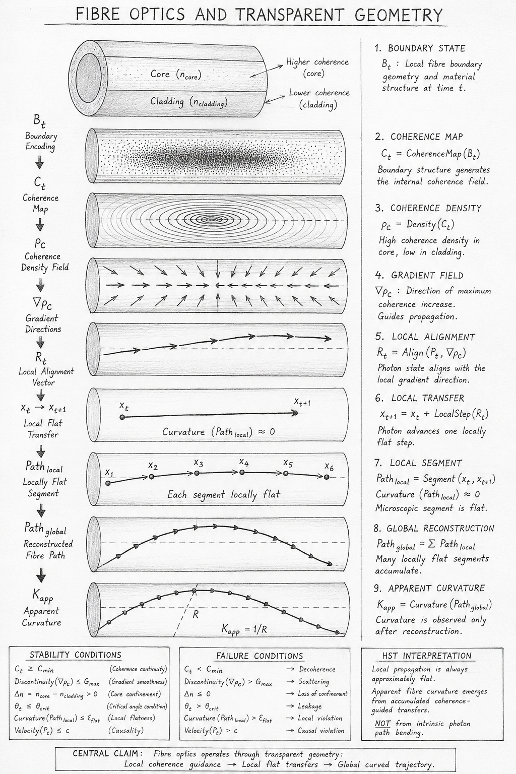
Overview of the Diagram

This diagram illustrates the HST interpretation of fibre optics as a coherence-guided propagation system. Rather than depicting photons physically bending through curved space or continuously refracting along a curved trajectory, the diagram demonstrates how apparent optical curvature emerges from the accumulation of many locally flat propagation events.

The figure follows the complete execution chain from boundary structure through coherence reconstruction, gradient formation, local alignment, microscopic transfer, and finally global trajectory reconstruction. Each layer corresponds directly to a stage in the Flow Algebra implementation and collectively demonstrates how transparent materials can guide propagation without requiring intrinsically curved photon motion.

Boundary State and Fibre Geometry

The upper section of the diagram begins with the optical fibre itself.

The fibre is separated into two distinct regions:

  • Core (ncoren_{core})
  • Cladding (ncladdingn_{cladding})

The core possesses the higher coherence density while the surrounding cladding possesses a lower coherence density.

This distinction creates the fundamental guidance mechanism of the fibre.

In HST terminology, the fibre acts as a boundary system:

\[ B_t \]

which contains the local geometric and material information available to the propagating photon.

The diagram shows that propagation begins not with motion, but with boundary encoding.

Coherence Map Formation

The next section illustrates the generation of:

\[ C_t = \mathrm{CoherenceMap} \left( B_t \right) \]

This stage converts the fibre geometry into a structured coherence field.

The shaded central region indicates that coherence is strongest inside the fibre core.

The coherence map is not the photon path itself.

Instead, it represents the navigational structure through which propagation becomes possible.

The diagram deliberately depicts this layer as a distributed field rather than a trajectory, emphasising that geometry is reconstructed before motion occurs.

Coherence Density Field

The third layer introduces:

\[ \rho_C \]

the coherence-density field.

The concentric contour structures shown inside the fibre represent regions of equal coherence density.

Higher-density regions occupy the central core while lower-density regions extend toward the cladding.

These contours play a role analogous to topographic lines on a geographical map.

Just as water naturally follows gravitational gradients, photon propagation follows coherence gradients.

The density field therefore establishes the stability landscape that governs subsequent propagation.

Gradient Field Formation

The next section depicts:

\[ \nabla \rho_C \]

through a collection of directional arrows.

These arrows indicate the direction of maximum coherence increase.

Within HST, gradients are the primary source of propagation guidance.

The photon does not calculate a complete future path.

Instead, it only evaluates local coherence conditions.

The gradient field therefore acts as a continuously updated directional instruction set.

This layer is critical because it transforms static coherence density into dynamic propagation guidance.

Local Alignment Vector

The diagram next introduces:

\[ R_t = \mathrm{Align} \left( P_t, \nabla \rho_C \right) \]

represented by the curved sequence of directional arrows.

The photon state aligns with the locally available coherence gradient.

Importantly, this alignment is local rather than global.

The photon has no knowledge of the overall fibre shape.

It simply selects the most coherent direction available at each instant.

This section visually communicates one of the core ideas of HST:

Propagation emerges from recursive local decisions rather than predetermined global trajectories.

Local Flat Transfer

The following layer depicts:

\[ x_{t+1} = x_t + \mathrm{LocalStep} \left( R_t \right) \]

with a straight transfer line connecting xtx_t and xt+1x_{t+1}.

The accompanying annotation:

\[ \mathrm{Curvature} \left( \mathrm{Path}_{\mathrm{local}} \right) \approx 0 \]

is one of the most important statements in the entire diagram.

It asserts that each individual propagation event remains locally flat.

No microscopic segment contains significant curvature.

This differs fundamentally from conventional interpretations that often treat the path as continuously curved at all scales.

Within HST, curvature does not exist at the transfer level.

Sequential Local Segments

The next panel expands this concept.

A chain of points:

\[ x_1 \rightarrow x_2 \rightarrow x_3 \rightarrow x_4 \rightarrow x_5 \rightarrow x_6 \]

shows multiple propagation updates.

Each segment remains individually flat.

The diagram emphasises:

Each segment locally flat.

This section demonstrates how complex propagation can emerge from repeated execution of simple transfer rules.

The process is entirely recursive.

Each update depends only on local coherence information generated by the previous state.

Global Fibre Path Reconstruction

The lower portion of the figure combines all local segments into:

\[ \mathrm{Path}_{\mathrm{global}} = \sum \mathrm{Path}_{\mathrm{local}} \]

The reconstructed path now appears curved.

This is the first location in the entire execution chain where observable curvature emerges.

The curve is not generated directly.

Instead, it is reconstructed from the accumulation of microscopic straight transfers.

The diagram therefore separates:

  • Local geometry
  • Global geometry

as distinct concepts.

This distinction is central to the HST interpretation.

Apparent Curvature

The final geometric panel introduces:

\[ K_{\mathrm{app}} = \mathrm{Curvature} \left( \mathrm{Path}_{\mathrm{global}} \right) \]

and illustrates a radius-of-curvature measurement:

\[ K_{\mathrm{app}} = \frac{R}{1} \]

The observer measures a curved fibre trajectory and infers curvature.

However, HST argues that this curvature exists only at the reconstruction level.

The local transfer events remain approximately flat throughout the process.

The figure therefore visually separates:

\[ \mathrm{Path}_{\mathrm{local}} \]

from

\[ \mathrm{Path}_{\mathrm{global}} \]

showing that curvature is an emergent property rather than a fundamental one.

Stability Conditions Panel

The lower-left panel lists the invariants required for stable propagation.

These include:

Coherence Continuity

\[ C_t \geq C_{\mathrm{min}} \]

Gradient Smoothness

\[ \mathrm{Discontinuity} \left( \nabla \rho_C \right) \leq G_{\mathrm{max}} \]

Core Confinement

\[ \Delta n = n_{\mathrm{core}} - n_{\mathrm{cladding}} > 0 \]

Critical Angle Preservation

\[ \theta_t \leq \theta_{\mathrm{crit}} \]

Local Flatness

Curvature(Pathlocal​)≤ϵflat​

Causal Consistency

\[ \mathrm{Velocity} \left( P_t \right) \leq c \]

These conditions define the operational envelope within which guided propagation remains stable.

Failure Conditions Panel

The centre-lower panel illustrates the mechanisms that terminate propagation.

Examples include:

\[ C_t < C_{\mathrm{min}} \]

leading to decoherence,

\[ \mathrm{Discontinuity} \left( \nabla \rho_C \right) > G_{\mathrm{max}} \]

leading to scattering,

and

\[ \Delta n \leq 0 \]

leading to loss of confinement.

This section demonstrates that fibre guidance is not guaranteed but emerges only when coherence-preserving conditions are maintained.

HST Interpretation Panel

The final panel summarises the conceptual conclusion of the entire chapter.

The diagram states:

\[ \mathrm{Path}_{\mathrm{local}} \approx \mathrm{Flat} \]

while simultaneously showing:

\[ \mathrm{Path}_{\mathrm{global}} \approx \mathrm{Curved} \]

The apparent contradiction is resolved by recognising that global curvature is a reconstruction effect arising from accumulated local transfers.

Within HST, the optical fibre does not bend photons through intrinsically curved trajectories.

Instead, it continuously realigns locally flat propagation events through structured coherence gradients generated by transparent boundary geometry.


Scientific Conclusion

The diagram provides a complete visual execution model of fibre-optic propagation within the Holographic Space-Time framework.

Beginning with boundary structure, it reconstructs coherence fields, generates density gradients, aligns photon propagation, executes locally flat transfer events, and accumulates those events into a globally curved trajectory.

The central result is that the observed curvature of optical fibres emerges from recursive coherence-guided alignment rather than fundamental photon-path bending. The figure therefore serves as a concrete demonstration of one of the core geometric principles of HST:

\[ \mathrm{Local\ Propagation} \approx \mathrm{Flat} \]

\[ \mathrm{Global\ Reconstruction} \approx \mathrm{Curved} \]

with curvature emerging from accumulated coherence-guided transfers through transparent geometry.

Scientific Mapping Between Diagram Elements and Flow Algebra

Diagram Element Flow Algebra Component Scientific Meaning
Fibre core and cladding cross-section B_t Physical boundary structure containing optical geometry
Core coherence label (n_core) n_core Higher coherence-density propagation channel
Cladding coherence label (n_cladding) n_cladding Lower coherence-density confinement region
Boundary encoding arrow C_t = CoherenceMap(B_t,n_core,n_cladding) Fibre geometry converted into a coherence field
Coherence field cylinder C_t Internal propagation landscape generated by boundary structure
Density cloud inside fibre ρ_C = Density(C_t) Distribution of coherence stability throughout the fibre
Density contours ρ_C Regions of equal coherence density
Gradient arrows ∇ρ_C Local directions of maximum coherence increase
Core–cladding contrast Δn = n_core - n_cladding Confinement mechanism maintaining guided propagation
Alignment vector panel R_t = Align(P_t,∇ρ_C) Local propagation direction selected from coherence geometry
Curved alignment arrows R_t Continuous local realignment process
Photon state P_t Current propagation configuration
Local transfer segment x_t+1 = x_t + LocalStep(R_t) Single coherent propagation update
Straight transfer line Path_local Individual microscopic propagation segment
Flatness annotation Curvature(Path_local) ≤ ε_flat Local propagation remains approximately straight
Sequence of points x₁→x₂→x₃→x₄→x₅→x₆ Recursive execution loop Repeated local coherence-guided transfers
Multi-segment propagation chain Σ Path_local Accumulation of microscopic transfer events
Reconstructed fibre trajectory Path_global Global path emerging from local propagation steps
Large-scale curved path Path_global ≈ Curved Observer-reconstructed optical trajectory
Radius-of-curvature sketch K_app = Curvature(Path_global) Apparent curvature measurement
Curvature label K_app = 1/R K_app Emergent large-scale optical curvature
Stability conditions panel Invariants Requirements for successful propagation
Failure conditions panel Failure_States Conditions that terminate coherent transport
HST interpretation box Scientific_Claim Curvature emerges from local flat transfers
Central claim statement Execution(P_t) = GUIDED_PROPAGATION Successful fibre-optic coherence transport

Layer-by-Layer Mapping

Diagram Layer Flow Layer Interpretation
Fibre Geometry B_t Boundary information source
Coherence Reconstruction C_t Internal coherence field generation
Density Formation ρ_C Propagation stability landscape
Gradient Formation ∇ρ_C Directional guidance field
Local Alignment R_t Propagation steering mechanism
Transfer Execution x_t → x_t+1 Microscopic propagation event
Local Segment Path_local Locally flat transfer path
Recursive Accumulation Σ Path_local Construction of macroscopic trajectory
Global Reconstruction Path_global Emergent fibre path
Curvature Measurement K_app Observed optical curvature

Flow Chain Mapping

Diagram Sequence Flow Expression Physical Interpretation
Boundary Structure B_t Fibre geometry exists
Coherence Generation B_t → C_t Geometry produces coherence field
Density Generation C_t → ρ_C Stability landscape emerges
Gradient Formation ρ_C → ∇ρ_C Guidance information appears
Alignment ∇ρ_C → R_t Photon selects coherent direction
Local Transfer R_t → x_t+1 Flat propagation update occurs
Segment Creation x_t → x_t+1 Local path element formed
Path Accumulation Σ Path_local Local transfers accumulate
Global Reconstruction Path_global Large-scale trajectory emerges
Curvature Observation K_app Apparent optical bending measured

Invariant Mapping

Diagram Condition Flow Invariant Meaning
Coherence Continuity C_t ≥ C_min Sufficient coherence for propagation
Gradient Smoothness Discontinuity(∇ρ_C) ≤ G_max Stable directional guidance
Core Confinement Δn > 0 Core remains preferred channel
Critical Angle Condition θ_t ≤ θ_crit Fibre guidance maintained
Local Flatness Curvature(Path_local) ≤ ε_flat Microscopic propagation remains straight
Causal Limit Velocity(P_t) ≤ c Physical consistency maintained

Failure-State Mapping

Diagram Failure Flow Failure State Physical Outcome
Decoherence C_t < C_min Propagation collapses
Gradient Breakdown Discontinuity(∇ρ_C) > G_max Scattering occurs
Confinement Loss Δn ≤ 0 Fibre guidance fails
Critical Angle Violation θ_t > θ_crit Leakage from core
Curvature Violation Curvature(Path_local) > ε_flat HST local-flatness failure
Causal Violation Velocity(P_t) > c Execution terminates

Ultra-Compressed Scientist Summary

Diagram Object Flow Symbol HST Meaning
Fibre B_t Boundary geometry
Core n_core High-coherence channel
Cladding n_cladding Confinement region
Coherence Field C_t Internal propagation map
Density ρ_C Stability field
Gradient ∇ρ_C Guidance direction
Alignment R_t Local propagation vector
Transfer x_t+1 Microscopic motion
Segment Path_local Flat propagation element
Reconstruction Path_global Emergent fibre path
Curvature K_app Observer-inferred bending
Stable Fibre Execution(P_t)=GUIDED_PROPAGATION Successful coherence transport
HST Result Path_local ≈ Flat → Path_global ≈ Curved Apparent curvature emerges from accumulated local transfers

Execution Guarantee Statement

Formal Execution Guarantee

The Fibre Optics and Transparent Geometry Flow is a deterministic coherence-guided propagation system. Given identical boundary geometry, coherence conditions, material parameters, and initial photon state, the flow will always reconstruct the same propagation pathway and produce the same resulting optical trajectory.

Execution does not depend upon randomness, hidden variables, probabilistic branching, observer intervention, or external interpretation.

The propagation sequence is fully specified by the recursive coherence chain:

\[ B_t \rightarrow C_t \rightarrow \rho_C \rightarrow \nabla \rho_C \rightarrow R_t \rightarrow x_{t+1} \rightarrow \mathrm{Path}_{\mathrm{local}} \rightarrow \mathrm{Path}_{\mathrm{global}} \rightarrow K_{\mathrm{app}} \]

where every stage is uniquely determined by the preceding state.

Deterministic Boundary Reconstruction

For any valid fibre geometry:

\[ B_t \]

the coherence reconstruction process

\[ C_t = \mathrm{CoherenceMap} \left( B_t, n_{\mathrm{core}}, n_{\mathrm{cladding}} \right) \]

produces a unique coherence field.

No ambiguity exists in the reconstruction stage.

Identical boundary conditions always generate identical coherence maps.

Therefore:

\[ B_t^{(1)} = B_t^{(2)} \]

implies

\[ C_t^{(1)} = C_t^{(2)} \]

Deterministic Gradient Formation

The coherence density calculation:

\[ \rho_C = \mathrm{Density} \left( C_t \right) \]

and subsequent gradient generation:

\[ \nabla \rho_C = \mathrm{Gradient} \left( \rho_C \right) \]

are deterministic operations.

For any identical coherence field:

\[ C_t \]

the resulting density landscape and gradient structure remain identical.

Therefore:

\[ C_t^{(1)} = C_t^{(2)} \]

guarantees

\[ \nabla \rho_C^{(1)} = \nabla \rho_C^{(2)} \]

Deterministic Alignment

The alignment operation:

\[ R_t = \mathrm{Align} \left( P_t, \nabla \rho_C \right) \]

contains no stochastic selection process.

Given identical photon state:

\[ P_t \]

and identical gradient structure:

\[ \nabla \rho_C \]

the resulting alignment vector is uniquely defined.

Thus:

\[ \left( P_t, \nabla \rho_C \right) \]

always yields a single propagation direction:

\[ R_t \]

for the same execution state.

Deterministic Local Transfer

The propagation update:

\[ x_{t+1} = x_t + \mathrm{LocalStep} \left( R_t \right) \]

is deterministic.

Given:

  • identical starting position,
  • identical alignment vector,
  • identical local coherence field,

the resulting transfer position is uniquely determined.

Therefore:

\[ x_t^{(1)} = x_t^{(2)} \]

and

\[ R_t^{(1)} = R_t^{(2)} \]

guarantee:

\[ x_{t+1}^{(1)} = x_{t+1}^{(2)} \]

Deterministic Path Reconstruction

The global optical trajectory is defined by:

\[ \mathrm{Path}_{\mathrm{global}} = \sum \mathrm{Path}_{\mathrm{local}} \]

Since every local transfer segment is uniquely determined, the accumulated trajectory is likewise uniquely determined.

No alternative path can emerge from identical initial conditions.

Thus:

\[ \left\{ \mathrm{Path}_{\mathrm{local}} \right\}^{(1)} = \left\{ \mathrm{Path}_{\mathrm{local}} \right\}^{(2)} \]

guarantees:

\[ \mathrm{Path}_{\mathrm{global}}^{(1)} = \mathrm{Path}_{\mathrm{global}}^{(2)} \]

Deterministic Curvature Reconstruction

The apparent curvature calculation:

\[ K_{\mathrm{app}} = \mathrm{Curvature} \left( \mathrm{Path}_{\mathrm{global}} \right) \]

depends solely upon the reconstructed path.

Since the path itself is deterministic, the curvature measurement is deterministic.

Therefore:

\[ \mathrm{Path}_{\mathrm{global}}^{(1)} = \mathrm{Path}_{\mathrm{global}}^{(2)} \]

guarantees:

\[ K_{\mathrm{app}}^{(1)} = K_{\mathrm{app}}^{(2)} \]

Execution Validity Conditions

Successful execution is guaranteed whenever:

\[ C_t \geq C_{\mathrm{min}} \]

\[ \mathrm{Discontinuity} \left( \nabla \rho_C \right) \leq G_{\mathrm{max}} \]

\[ \Delta n = n_{\mathrm{core}} - n_{\mathrm{cladding}} > 0 \]

\[ \theta_t \leq \theta_{\mathrm{crit}} \]

\[ \mathrm{Curvature} \left( \mathrm{Path}_{\mathrm{local}} \right) \leq \epsilon_{\mathrm{flat}} \]

\[ \mathrm{Velocity} \left( P_t \right) \leq c \]

remain satisfied throughout execution.

Under these conditions:

\[ \mathrm{Execution} \left( P_t \right) = \mathrm{GUIDED\_PROPAGATION} \]

is guaranteed.

Failure Guarantee

The flow also guarantees deterministic failure behaviour.

If any invariant is violated:

\[ C_t < C_{\mathrm{min}} \]

or

\[ \mathrm{Discontinuity} \left( \nabla \rho_C \right) > G_{\mathrm{max}} \]

or

\[ \Delta n \leq 0 \]

or

\[ \theta_t > \theta_{\mathrm{crit}} \]

or

\[ \mathrm{Velocity} \left( P_t \right) > c \]

then execution transitions predictably into:

\[ \mathrm{Execution} \left( P_t \right) = \mathrm{FAIL} \]

No undefined intermediate state exists.

Failure conditions are completely specified by the flow.

Reproducibility Guarantee

For any two independent implementations executing the same flow:

\[ \left( B_t, n_{\mathrm{core}}, n_{\mathrm{cladding}}, P_t, x_t \right) \]

with identical parameters and thresholds, the resulting outputs:

\[ \mathrm{Path}_{\mathrm{global}} \]

and

\[ K_{\mathrm{app}} \]

must be identical.

Therefore the flow is:

  • Deterministic
  • Reproducible
  • Platform-independent
  • Observer-independent
  • Recursively executable
  • Zero-shot deployable

under the Flow Algebra framework.

Formal Guarantee Statement

\[ B_t \rightarrow C_t \rightarrow \rho_C \rightarrow \nabla \rho_C \rightarrow R_t \rightarrow x_{t+1} \rightarrow \mathrm{Path}_{\mathrm{global}} \rightarrow K_{\mathrm{app}} \]

If all invariants remain satisfied, the flow is guaranteed to produce a unique, reproducible, and stable fibre-optic propagation trajectory.

Under HST, the resulting optical path emerges from deterministic sequences of locally flat coherence-guided transfers, yielding an observer-reconstructed global curvature without requiring intrinsically curved photon motion.

This execution guarantee holds for every valid state satisfying the flow constraints.

Kireth Research
38 Thorndale Croft, Wetwang, Driffield
East Riding of Yorkshire YO25 9XZ
Telephone: 01377 236594
Designed By