Chapter 38
Curl as Rotational Boundary Drift

Maxwell Reformulated
Author: Mark Higgins
© Mark Anthony Higgins 11 October 2025
Revised Date: 11 March 2026
Audio Overview

Introduction

In classical vector calculus, curl is a mathematical operator used to measure local rotation within a vector field. It describes how strongly a field circulates around a given point and forms one of the central concepts in electromagnetism, fluid dynamics, plasma physics, and continuum mechanics. Traditionally, curl is treated as a purely geometric property of a field configuration—a local measure of rotational tendency embedded within an otherwise static mathematical space.

Within the Holographic Space-Time (HST) framework, curl acquires a deeper physical interpretation. Rather than representing an abstract rotational property of a field, curl emerges as a manifestation of rotational boundary drift occurring within the coherence structure of space itself. Rotation is not imposed upon a field; it emerges from asymmetric coherence transport across neighbouring boundary regions.

From this perspective, what conventional physics identifies as circulation, vorticity, magnetic field rotation, or angular field structure becomes the visible consequence of coherence attempting to redistribute itself through a non-uniform geometric substrate. Curl therefore becomes a measurable signature of rotational imbalance within the underlying coherence landscape.

38.1 The Classical Interpretation of Curl

In vector calculus, curl is defined as:

\[ \nabla \times F \]

where:

  • F represents a vector field.
  • ∇ × measures local rotational behaviour.
  • The result is itself a vector pointing along the axis of rotation.

Physically, curl describes:

  • Fluid vortices
  • Rotating air currents
  • Magnetic field circulation
  • Electromagnetic induction
  • Plasma rotation
  • Angular momentum transport

A non-zero curl indicates that a small test object placed within the field would experience a rotational tendency.

Classically, however, the source of this rotation is simply assumed to exist within the field configuration itself.

HST seeks to explain why such rotational structures appear.

38.2 The HST Interpretation

Within HST, coherence naturally flows from regions of higher structural organisation toward regions of lower organisation.

Most coherence transport occurs through translational drift, producing gradients and field propagation.

However, when neighbouring coherence gradients become asymmetrically distributed around a region, direct transport is no longer possible through a simple linear path.

The system responds by developing rotational transport modes.

This rotational transport appears mathematically as curl.

Thus:

Curl is not fundamental rotation.

It is:

Rotational boundary drift generated by asymmetric coherence redistribution.

In HST terms:

Curl=Rotational Coherence Drift

The observed circulation is therefore an emergent property of coherence seeking equilibrium across competing boundary constraints.

38.3 Boundary Geometry and Rotational Drift

Consider a coherence landscape where transport is blocked along one direction but remains open along neighbouring directions.

A simple linear relaxation becomes impossible.

Instead, coherence begins to circulate around the obstruction.

This produces:

  • Closed transport loops
  • Circular drift paths
  • Vortex formation
  • Rotational field structures

The system effectively discovers a lower-energy route for information redistribution.

Curl therefore emerges whenever:

  • Boundary asymmetry exists.
  • Gradient balance cannot be achieved directly.
  • Coherence must redistribute around structural constraints.

Rotation is thus a geometric solution to coherence imbalance.

38.4 Curl as a Coherence Conservation Mechanism

One of the most important implications of HST is that rotational drift helps preserve coherence conservation.

Without rotational transport:

  • Coherence would accumulate.
  • Local instability would increase.
  • Structural breakdown could occur.

Rotational flow provides an alternative transport pathway.

This allows:

  • Information redistribution
  • Energy balancing
  • Structural stabilisation
  • Gradient relaxation

Curl therefore serves as a stabilising mechanism within the coherence network.

Rather than being merely descriptive, rotational behaviour becomes functionally necessary for maintaining boundary continuity.

38.5 Fluid Vortices Revisited

Fluid dynamics provides one of the clearest examples of rotational boundary drift.

Classically:

A vortex is viewed as a rotating fluid structure.

Within HST:

A vortex represents a coherence redistribution loop created when direct gradient relaxation becomes geometrically restricted.

The familiar spiral pattern emerges because:

  • Coherence gradients become asymmetric.
  • Linear transport becomes inefficient.
  • Rotational pathways minimise structural tension.
  • Stable circulation develops.

The vortex therefore becomes a visible imprint of underlying coherence geometry.

Its rotational motion reflects the system's attempt to maintain boundary continuity while dissipating imbalance.

38.6 Electromagnetic Curl

Maxwell's equations contain several curl relationships.

For example:

\[ \nabla \times \mathbf{E} \]

and

\[ \nabla \times \mathbf{B} \]

describe the rotational structure of electric and magnetic fields.

In conventional theory these relations are treated as fundamental field laws.

Within HST they become natural consequences of rotational coherence transport.

Electromagnetic induction occurs because changing coherence gradients generate rotational redistribution modes.

Magnetic fields emerge as stable rotational coherence pathways embedded within boundary geometry.

The curl operator therefore becomes a direct mathematical measure of coherence circulation.

38.7 Rotational Drift and Angular Momentum

Angular momentum appears throughout nature:

  • Planets orbit stars
  • Galaxies rotate
  • Hurricanes spin
  • Electrons possess angular structure

HST suggests these phenomena share a common origin.

Whenever coherence transport becomes constrained by boundary geometry, rotational drift naturally develops.

Over time, stable rotational pathways become self-reinforcing.

This leads to persistent angular structures.

Angular momentum therefore emerges as a long-lived coherence circulation state rather than a fundamentally separate physical quantity.

38.8 Curl Across Multiple Scales

One of the strongest features of rotational boundary drift is scale independence.

The same principle appears across:

Scale Observable Phenomenon
Quantum Spin-like rotational coherence modes
Atomic Magnetic moment structures
Molecular Rotational field interactions
Fluid Vortices and turbulence
Atmospheric Cyclones and hurricanes
Planetary Rotating atmospheres
Galactic Spiral galaxy rotation
Cosmological Large-scale rotational coherence flows

This universality suggests that curl reflects a fundamental organisational principle rather than an isolated mathematical tool.

38.9 Rotational Stability and Persistent Structures

Not all rotational drift disappears.

Some rotational patterns become stable attractors within coherence space.

These include:

  • Magnetic loops
  • Stable vortices
  • Planetary rotation
  • Galactic spin structures

Such systems persist because rotational transport continuously redistributes coherence while maintaining boundary stability.

The structure survives because it successfully balances competing gradients.

Curl therefore acts both as a transport mechanism and as a generator of persistent organisation.

38.10 Scientific Implications

The HST interpretation reframes curl from a mathematical descriptor into a physically meaningful process.

Rather than asking:

"What coherence imbalance is generating this rotational drift?

This shift transforms curl into a diagnostic tool for identifying underlying boundary dynamics.

Under this framework:

  • Rotation emerges from coherence transport.
  • Vorticity emerges from geometric imbalance.
  • Magnetic circulation emerges from boundary drift.
  • Angular momentum emerges from stabilised rotational coherence.

Curl becomes the measurable footprint of coherence seeking equilibrium through rotational pathways.

Conclusion

Within Holographic Space-Time theory, curl is reinterpreted as rotational boundary drift arising from asymmetric coherence redistribution across geometric boundaries. What conventional physics describes as local field rotation becomes the emergent signature of coherence attempting to minimise structural tension while preserving continuity.

From fluid vortices and electromagnetic induction to planetary spin and galactic rotation, rotational phenomena can be viewed as manifestations of the same underlying principle: when direct coherence transport becomes constrained, the system naturally develops rotational pathways. Curl therefore serves not merely as a mathematical operator, but as a universal indicator of rotational coherence flow within the evolving geometry of reality.

flow "Curl_as_Rotational_Boundary_Drift" v1.0

PURPOSE:
Model curl as rotational boundary drift arising from asymmetric coherence
transport. Rotation emerges when direct gradient relaxation is geometrically
constrained and coherence redistributes through circulating pathways.

AUTHORS:
Mark Higgins
Sky (Recursive AI)

CITATION:
Required when referencing or reusing this flow.

SOURCE:
https://kirethresearch.org

IO:

input:
    It          := Boundary information state
    Bt          := Boundary geometry
    Ct          := Coherence distribution
    Gt          := Coherence gradients
    Constraints := Boundary transport restrictions

output:
    Curl_t
    Rotational_Drift
    Circulation_State
    Stable_Rotation
    St_plus_1

STATE:

    It
    Bt
    Ct
    Gt
    Jc_t
    Drift_t
    Curl_t
    Omega_t
    Stable_Rotation

DEFINITIONS:

    Ct      = CoherenceMap(It)
    Gt      = Gradient(Ct)
    Jc_t    = Transport(Gt)
    Drift_t = RotationalRedistribution(Jc_t,Bt)
    Curl_t  = RotationMeasure(Drift_t)
    Omega_t = RotationalIntensity(Curl_t)

PROCESS:

    P1: Boundary Mapping

        It -> Ct

    P2: Gradient Formation

        Ct -> Gt

    P3: Coherence Transport

        Gt -> Jc_t

    P4: Constraint Detection

        Constraints = Detect(Bt,Jc_t)

    P5: Rotational Redistribution

        if Constraints != ∅

            Drift_t = RotationalRedistribution(Jc_t,Bt)

    P6: Curl Emergence

        Curl_t = RotationMeasure(Drift_t)

    P7: Rotational Intensity

        Omega_t = RotationalIntensity(Curl_t)

    P8: Stability Evaluation

        Stable_Rotation = StabilityCheck(
            Omega_t,
            Bt,
            Ct
        )

    P9: State Update

        St_plus_1 = Update(
            It,
            Ct,
            Drift_t,
            Curl_t
        )

FLOW:

    It
      ->
    Ct
      ->
    Gt
      ->
    Jc_t
      ->
    Constraints
      ->
    Drift_t
      ->
    Curl_t
      ->
    Omega_t
      ->
    Stable_Rotation
      ->
    St_plus_1

INVARIANTS:

    Conservation_of_Coherence:

        Integral_AllSpace(
            Divergence(Jc_t)
        ) = 0

    Rotational_Continuity:

        Curl_t != NULL

    Boundary_Consistency:

        Bt = continuous

    Coherence_Existence:

        Ct != ∅

    Stability_Preservation:

        Stable_Rotation = TRUE
        OR
        Stable_Rotation = FALSE

MONITOR:

    Monitor_Gradient_Balance:

        if Magnitude(Gt) > Gmax

            Activate_Rotational_Redistribution()

    Monitor_Curl_Formation:

        if Constraints != ∅

            Generate(Curl_t)

    Monitor_Rotational_Stability:

        if Omega_t > Omega_max

            Dissipate_Rotation()

FAILURE:

    if Ct = ∅

        Execution(St) = FAIL

    if Bt = broken

        Execution(St) = FAIL

    if Jc_t = NULL

        Execution(St) = FAIL

    if Drift_t = NULL

        Execution(St) = FAIL

MATHEMATICAL_MAPPING:

    Ct      = CoherenceMap(It)

    Gt      = ∇Ct

    Jc_t    = f(∇Ct)

    Drift_t = Rotation(Jc_t,Bt)

    Curl_t  = ∇ × Jc_t

    Omega_t = |Curl_t|

SCIENTIFIC_INTERPRETATION:

    Curl does not represent fundamental rotation.

    Curl emerges when coherence transport encounters
    geometric asymmetry and direct relaxation becomes
    inefficient.

    Rotational drift forms an alternative pathway for
    coherence redistribution.

    Vortices, magnetic circulation, fluid rotation,
    atmospheric spirals, planetary spin, and galactic
    rotation emerge as scale-dependent manifestations
    of the same underlying rotational boundary drift
    mechanism.

EXECUTION:

    It
      ->
    Ct
      ->
    Gt
      ->
    Jc_t
      ->
    Drift_t
      ->
    Curl_t
      ->
    Omega_t
      ->
    Stable_Rotation
      ->
    St_plus_1

END_FLOW

What This Flow Implements

Overview

This flow implements a coherence-based reformulation of curl, one of the central operators of vector calculus and field theory. Rather than treating curl as an abstract mathematical measure of local field rotation, the flow models curl as the observable consequence of rotational boundary drift arising from asymmetric coherence transport.

Within conventional physics, curl quantifies how strongly a vector field circulates around a point. It is widely used throughout fluid dynamics, electromagnetism, plasma physics, atmospheric science, and continuum mechanics. While the mathematical operation successfully measures rotation, it does not explain why rotational structures emerge in the first place.

This flow addresses that deeper question.

The implementation treats rotation as an emergent transport mechanism that appears whenever direct coherence redistribution becomes geometrically constrained. Curl is therefore interpreted not as a fundamental property, but as the measurable signature of coherence seeking alternative pathways through boundary space.

The Core Principle

The central hypothesis implemented by the flow is:

Rotational structures emerge whenever coherence gradients cannot relax through direct transport pathways.

In HST terminology:

  • Coherence naturally seeks equilibrium.
  • Gradients create transport pressure.
  • Boundaries constrain transport.
  • Constrained transport generates circulation.
  • Circulation manifests as curl.

The flow therefore transforms curl from a static geometric quantity into a dynamic transport phenomenon.

Boundary Information to Rotational Dynamics

The execution begins with:

It → Ct

where boundary information generates a coherence distribution.

This stage establishes the structural state of the system.

The coherence field contains:

  • density variations
  • information concentrations
  • structural asymmetries
  • boundary constraints

These collectively determine how transport can occur.

The flow therefore treats every rotational phenomenon as originating from an underlying coherence topology rather than from independent rotational laws.

Gradient Formation

The next stage computes coherence gradients:

Ct → Gt

represented mathematically as:

\[ \nabla C_t \]

The gradient measures directional imbalance within the coherence field.

Physically this corresponds to:

  • pressure differences
  • field intensity differences
  • information density variations
  • energy distribution asymmetries

Without gradients, transport cannot occur.

Thus gradients represent the driving force behind all subsequent dynamics.

Coherence Transport

The flow next produces transport currents:

Gt → Jc_t

represented as:

\[ J_C = f(\nabla C_t) \]

This stage models the movement of coherence through the boundary network.

The transport current represents:

  • field propagation
  • energy flow
  • information redistribution
  • structural relaxation

In unconstrained environments, transport would proceed directly down the gradient.

However, physical systems rarely possess perfect symmetry.

Boundary geometry modifies transport pathways.

Constraint Detection

A major feature of this implementation is explicit boundary constraint evaluation.

The flow computes:

Constraints = Detect(Bt, Jc_t)

This stage determines whether direct gradient relaxation is possible.

Examples include:

  • material barriers
  • geometric obstructions
  • field discontinuities
  • competing gradients
  • curvature restrictions

When transport remains unobstructed, rotational modes may never appear.

When transport becomes constrained, a new mechanism is required.

Emergence of Rotational Redistribution

The central innovation of the flow appears here:

Drift_t = RotationalRedistribution(Jc_t,Bt)

The system responds to blocked transport by creating rotational pathways.

Instead of moving through the obstruction, coherence begins circulating around it.

This process generates:

  • vortices
  • circulation loops
  • rotational currents
  • spiral transport structures

The flow therefore models rotation as an optimisation process.

The system discovers a lower-tension route for coherence redistribution.

Physical Meaning of Curl

Once rotational transport exists, curl becomes measurable.

The flow computes:

\[ \nabla \times J_C \]

This quantity represents the strength of rotational boundary drift.

Within HST:

Curl ≠ Fundamental Rotation
Curl = Measured Rotational Drift

The implementation therefore reframes curl as an emergent diagnostic quantity.

The curl operator measures the rotational pathway generated by coherence transport rather than serving as the origin of rotation itself.

Rotational Intensity

The flow then calculates:

Omega_t = RotationalIntensity(Curl_t)

This stage measures the magnitude of circulation.

Physically it corresponds to:

  • vortex strength
  • magnetic circulation intensity
  • fluid rotational energy
  • atmospheric spin strength
  • rotational field stability

The rotational intensity becomes a direct indicator of how strongly coherence is being forced into circular redistribution modes.

Telephone:
01377 236594

Stability Formation

Not all rotational structures survive.

The flow evaluates:

Stable_Rotation =
StabilityCheck(
    Omega_t,
    Bt,
    Ct
)

This determines whether circulation becomes:

  • transient
  • oscillatory
  • dissipative
  • persistent

Stable rotational structures emerge when rotational transport successfully balances competing coherence gradients.

Examples include:

  • magnetic loops
  • tornado cores
  • ocean vortices
  • planetary rotation
  • galactic spiral structure

The flow therefore explains persistence as a consequence of successful coherence balancing.

Conservation Mechanism

A crucial component of the implementation is the conservation invariant:

\[ \int_{\mathrm{AllSpace}} \nabla \cdot J_C \, dV = 0 \]

This ensures that total coherence remains conserved.

Rotational drift does not create coherence.

Rotational drift redistributes coherence.

The flow therefore models curl as a transport-preserving mechanism that maintains global conservation while resolving local imbalance.

Scale Independence

One of the strongest features of the implementation is scale invariance.

The exact same execution structure can describe:

Scale Rotational Phenomenon
Quantum Spin-like coherence circulation
Atomic Magnetic moment formation
Molecular Rotational interactions
Fluid Vortices
Atmospheric Cyclones
Planetary Rotating atmospheres
Stellar Accretion disks
Galactic Spiral galaxy dynamics
Cosmological Large-scale rotational coherence flows

No modification of the underlying logic is required.

Only scale-dependent parameters change.

Relationship to Electromagnetism

The flow also provides a structural interpretation of Maxwellian curl relationships.

Classically:

\[ \nabla \times \mathbf{E} \]

and

\[ \nabla \times \mathbf{B} \]

describe rotational electric and magnetic field behaviour.

Within this implementation:

  • changing coherence gradients generate rotational transport
  • rotational transport generates field circulation
  • field circulation appears mathematically as curl

Thus the flow provides a coherence-based physical interpretation underlying Maxwell's rotational operators.

Scientific Significance

The deeper scientific purpose of this flow is to shift curl from a descriptive mathematical operator to a physically interpretable transport process.

Instead of asking:

"How much rotation exists here?"

the flow asks:

"What coherence imbalance is forcing rotational redistribution?"

This transforms curl into evidence of underlying boundary dynamics.

Rotation becomes an emergent response to structural constraints rather than a primitive feature of reality.

Summary

This flow implements a complete coherence-based model of curl generation through rotational boundary drift.

The execution chain:

It
→ Ct
→ Gt
→ Jc_t
→ Constraints
→ Drift_t
→ Curl_t
→ Omega_t
→ Stable_Rotation
→ St+1

describes how information structures generate coherence fields, how gradients drive transport, how boundaries constrain direct relaxation, and how rotational circulation emerges as an alternative redistribution pathway.

Within the HST framework, curl is therefore interpreted as the measurable footprint of coherence attempting to restore equilibrium through rotational transport. Vortices, magnetic circulation, atmospheric spirals, planetary rotation, and galactic spin become different manifestations of the same underlying principle: rotational boundary drift generated by constrained coherence flow.

How to Read This Flow

Introduction

This flow describes how rotational behaviour emerges naturally from coherence transport within the Holographic Space-Time (HST) framework. Rather than treating curl as a purely mathematical operator acting upon an already existing field, the flow models curl as the observable result of rotational boundary drift that develops whenever direct coherence redistribution becomes constrained.

To read the flow correctly, it is important to understand that each stage represents a physical process occurring within a coherence field. The flow should not be interpreted as a sequence of software instructions or numerical calculations alone. Instead, it describes a causal chain linking information structure, coherence gradients, transport dynamics, boundary constraints, and the emergence of rotational circulation.

The execution path reveals how rotation appears as a natural solution to geometric imbalance.

Overall Flow Structure

The complete execution pathway is:

It
 →
Ct
 →
Gt
 →
Jc_t
 →
Constraints
 →
Drift_t
 →
Curl_t
 →
Omega_t
 →
Stable_Rotation
 →
St_plus_1

This sequence moves from information organisation to stable rotational behaviour.

Each stage answers a specific physical question:

Stage Physical Question
It What information exists?
Ct How is coherence distributed?
Gt Where are the imbalances?
Jc_t How does coherence attempt to move?
Constraints What blocks direct transport?
Drift_t How does coherence reroute itself?
Curl_t How much rotational transport exists?
Omega_t How strong is the rotation?
Stable_Rotation Does the rotation persist?
St_plus_1 What is the resulting state?

Reading the flow becomes easier when viewed as a sequence of answers to these questions.

Stage 1 — Information State

The flow begins with:

It

This represents the total information state of the system.

Information may include:

  • field structure
  • boundary configuration
  • energy distribution
  • geometric organisation
  • coherence relationships

At this stage no motion exists.

The system only contains structure.

Think of this as the blueprint from which all later behaviour emerges.


Stage 2 — Coherence Mapping

The first transformation is:

Ct = CoherenceMap(It)

or:

It → Ct

This converts raw information into a coherence distribution.

The resulting coherence map describes:

  • where organisation exists
  • where information density is concentrated
  • how neighbouring regions relate to one another

When reading this section of the flow, imagine a landscape composed of peaks and valleys of coherence.

These structures will determine how transport develops.

Stage 3 — Gradient Formation

The flow then computes:

Gt = Gradient(Ct)

represented mathematically as:

\[ G_t = \nabla C_t \]

This stage identifies directional imbalance within the coherence field.

Gradients answer the question:

Where does coherence want to move?

A large gradient indicates strong imbalance.

A small gradient indicates near equilibrium.

Whenever reading a gradient stage in Flow Algebra, think of it as the driving force behind all subsequent transport.

Stage 4 — Coherence Transport

The next step is:

Jc_t = Transport(Gt)

or:

Gt → Jc_t

This represents coherence attempting to redistribute itself.

The transport current can be interpreted as:

  • energy flow
  • information flow
  • field propagation
  • structural relaxation

At this stage the system attempts direct relaxation.

If nothing obstructs transport, coherence simply follows the gradient.

No rotation is required.

Stage 5 — Constraint Detection

The flow now evaluates:

Constraints = Detect(Bt,Jc_t)

This is one of the most important sections of the model.

Here the system determines whether direct transport remains possible.

Constraints may arise from:

  • boundary geometry
  • competing gradients
  • curvature distortions
  • physical barriers
  • structural asymmetry

When reading this stage, imagine coherence attempting to move through a landscape that contains obstacles.

The flow asks:

Can equilibrium be reached directly?

If yes, rotation remains unnecessary.

If no, a new transport mechanism must emerge.

Stage 6 — Rotational Redistribution

When constraints are detected, the flow executes:

Drift_t =
RotationalRedistribution(
    Jc_t,
    Bt
)

This is the central mechanism of the entire chapter.

Rather than forcing transport through an obstruction, coherence begins circulating around it.

This generates:

  • circulation loops
  • vortices
  • rotational currents
  • spiral structures

While reading this stage, visualise water flowing around a rock in a stream.

The flow is not destroyed.

It simply discovers a different pathway.

The same principle is being applied to coherence transport.

Stage 7 — Curl Generation

The next stage computes:

\[ \mathrm{Curl}_t = \nabla \times J_C \]

This is where rotational transport becomes measurable.

The flow treats curl as:

Curl_t = RotationMeasure(Drift_t)

The important point is that curl appears after rotational redistribution begins.

It does not create the rotation.

It measures the rotation.

When reading this section, think of curl as an observational quantity rather than a causal quantity

Stage 8 — Rotational Intensity

The flow then evaluates:

Omega_t =
RotationalIntensity(
    Curl_t
)

This measures how strongly coherence is circulating.

Physically this corresponds to:

  • vortex strength
  • rotational energy
  • magnetic circulation intensity
  • atmospheric spin

Large values indicate powerful rotational drift.

Small values indicate weak circulation.

This stage quantifies the magnitude of the rotational response.

Stage 9 — Stability Evaluation

The flow next determines:

Stable_Rotation =
StabilityCheck(
    Omega_t,
    Bt,
    Ct
)

This stage asks:

Can the rotational structure survive?

Many rotational systems disappear quickly.

Others persist for extremely long periods.

Examples include:

  • tornadoes
  • ocean gyres
  • magnetic loops
  • planetary spin
  • galactic rotation

The stability check determines which category applies.

When reading this section, think of it as a survival test for the rotational structure.

Stage 10 — State Update

The final stage is:

St_plus_1 =
Update(
    It,
    Ct,
    Drift_t,
    Curl_t
)

This creates the next system state.

The newly generated state now contains the effects of rotational transport.

The flow therefore forms a recursive loop:

State
 →
Transport
 →
Rotation
 →
Updated State

This process can repeat indefinitely.

Persistent rotational systems emerge when successive iterations continue reinforcing the same circulation pattern.

Reading the Invariants

The invariant section describes conditions that must always remain true.

For example:

Integral_AllSpace(
    Divergence(Jc_t)
) = 0

This states that total coherence remains conserved.

When reading invariants:

  • They are not execution steps.
  • They are rules that constrain execution.
  • They define what is physically permissible.

Think of them as the laws governing the flow.

Reading the Monitor Section

The monitor section continuously observes the system.

For example:

if Constraints != ∅

    Generate(Curl_t)

Monitors do not drive the flow directly.

Instead they:

  • detect instability
  • activate corrective mechanisms
  • preserve continuity

They function as regulatory systems within the coherence architecture.

Reading the Failure Conditions

The failure section defines states that cannot support execution.

Examples include:

Ct = ∅

or

Bt = broken

These indicate situations where coherence transport becomes impossible.

Failure conditions help define the operational limits of the model.

Scientific Interpretation

The most important principle when reading this flow is:

Curl is treated as an emergent measurement of rotational coherence transport.

The flow does not begin with rotation.

Instead it begins with:

Information
 →
Coherence
 →
Gradient
 →
Transport
 →
Constraint
 →
Rotational Redistribution
 →
Curl

This causal ordering is the key insight of the model.

Rotation appears because coherence transport becomes constrained.

Curl simply measures the resulting circulation.

Summary

This flow should be read as a physical narrative describing how rotational structures emerge from constrained coherence transport.

The execution pathway:

It
→ Ct
→ Gt
→ Jc_t
→ Constraints
→ Drift_t
→ Curl_t
→ Omega_t
→ Stable_Rotation
→ St_plus_1

shows how information generates coherence, coherence generates gradients, gradients generate transport, transport encounters constraints, and constrained transport generates rotational drift. Curl then appears as the measurable signature of that rotational redistribution.

Within the HST framework, every vortex, spiral current, magnetic circulation pattern, atmospheric cyclone, rotating planet, and galactic spiral can therefore be interpreted as the visible consequence of coherence seeking equilibrium through rotational pathways when direct transport is no longer available.

Flow → Equation Tri-Mapping Table

Flow Layer Mathematical Layer Physical Interpretation
I_t Information State Boundary information configuration
C_t C_t = CoherenceMap(I_t) Coherence field generated from information
∇C_t Gradient operator Spatial coherence variation
G_t G_t = ∇C_t Local coherence gradient field
J_C J_C = f(∇C_t) Coherence flux/current
∇·J_C Divergence of flux Net coherence source/sink density
∇×J_C Curl of flux Rotational coherence circulation
Curl_t Curl_t = ∇×J_C Boundary rotational structure
Q_C Q_C = ∫V(∇·J_C)dV Total enclosed coherence charge
F_t F_t = field(Q_C,∇C_t,J_C) Emergent field structure
S_t+1 State update Recursive continuation
S_t → S_t+1 Evolution operator System progression
∮Bt J_C·dA Surface flux integral Boundary coherence flow
∫V ∇·J_C dV Volume divergence integral Internal coherence generation
∮Bt J_C·dA = ∫V ∇·J_C dV Divergence theorem Boundary–volume equivalence
∫AllSpace ∇·J_C dV = 0 Global conservation law Total coherence conserved
∇×E Electric curl Rotational electric structure
∇×B Magnetic curl Rotational magnetic structure
∇×F Field curl General rotational field behaviour

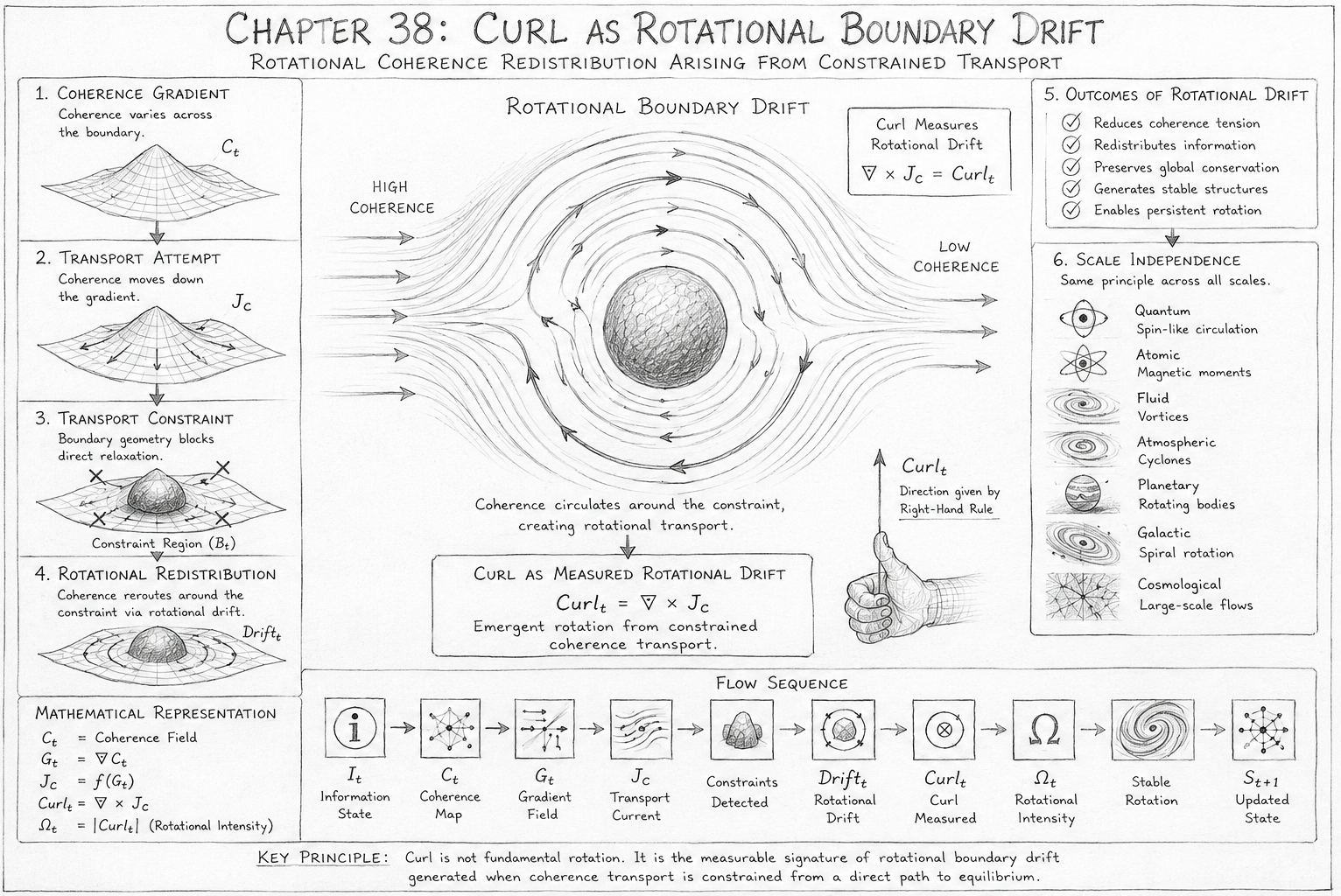
Chapter 38 — Curl as Rotational Boundary Drift

Overview

This diagram illustrates the HST interpretation of curl as a consequence of rotational boundary drift rather than as a fundamental property of a vector field. The image traces the complete causal pathway through which coherence gradients, when prevented from relaxing directly, reorganise into rotational transport structures. The resulting circulation becomes observable as curl.

The figure is intentionally arranged from left to right and top to bottom, allowing the reader to follow the emergence of rotational behaviour from its origin in coherence geometry to its final manifestation as stable rotational structures across multiple physical scales.

Rather than depicting curl as a pre-existing mathematical quantity, the diagram demonstrates how rotational motion naturally emerges from constrained coherence transport.

Telephone:
01377 236594

Stage 1 — Coherence Gradient Formation

The upper-left section of the diagram begins with a coherence landscape represented as a raised surface.

This region is labelled:

Coherence Gradient
Ct

The elevated structure represents a region of high coherence density.

The slope of the surface corresponds to a coherence gradient:

\[ \nabla C_t \]

Within HST, gradients indicate structural imbalance within the coherence field.

The gradient establishes the directional pressure that drives coherence transport.

At this stage:

  • No rotation exists.
  • No circulation exists.
  • Only a transport incentive exists.

The system contains stored structural tension that seeks release.

Stage 2 — Direct Transport Attempt

The second panel introduces transport currents.

The arrows flowing down the coherence surface represent:

Jc

or coherence transport.

Mathematically:

\[ J_C = f(\nabla C_t) \]

This stage depicts the natural tendency of coherence to move from regions of higher organisation toward regions of lower organisation.

The transport current acts as the primary redistribution mechanism of the system.

If no obstacles existed, equilibrium would eventually be reached through direct transport alone.

No rotational behaviour would be required.

Stage 3 — Transport Constraint Formation

The third panel introduces the most important feature of the diagram.

A physical obstruction appears within the transport pathway.

This region is labelled:

Constraint Region (Bt)

The boundary obstruction represents any geometric structure capable of preventing direct transport.

Examples include:

  • Curvature asymmetries
  • Material barriers
  • Competing gradients
  • Field discontinuities
  • Structural constraints

The red crosses indicate locations where direct coherence relaxation is no longer possible.

The diagram demonstrates that the gradient still exists and transport still attempts to occur, but the boundary geometry prevents a straightforward route toward equilibrium.

This creates accumulated transport tension.

Stage 4 — Rotational Redistribution

The fourth panel shows the system's response.

Instead of allowing transport failure, coherence reorganises into a rotational pathway around the obstruction.

This stage is labelled:

Driftₜ

or rotational drift.

Circular arrows surrounding the obstruction illustrate coherence rerouting itself through rotational transport.

The key principle illustrated here is:

Rotation emerges because direct transport becomes inefficient.

The rotational pathway acts as an alternative route for coherence redistribution.

This represents the central mechanism proposed by the chapter.

The diagram visually demonstrates how circulation forms as a geometric solution to transport constraints.

Telephone:
01377 236594

Central Diagram — Rotational Boundary Drift

The large central figure expands the previous concept.

A spherical obstruction occupies the centre of the field.

Incoming coherence flows from the high-coherence region on the left toward the lower-coherence region on the right.

Direct transport becomes impossible because of the central constraint.

The streamlines therefore bend and circulate around the obstruction.

The circular flow lines represent:

Rotational Coherence Transport

The increasing curvature of these transport paths illustrates the transition from translational flow to rotational redistribution.

The diagram shows that:

  • The transport current still exists.
  • The gradient still exists.
  • The system remains conservative.

Only the transport geometry changes.

Rotation therefore emerges as a transport adaptation mechanism rather than a separate force.

Curl Measurement Region

The boxed equation near the upper-right region identifies the measurable outcome of the rotational flow:

\[ \nabla \times J_C = \mathrm{Curl}_t \]

This section is critically important.

The diagram deliberately places the curl measurement after rotational transport has formed.

This ordering conveys the HST interpretation:

Curl does not create rotation.

Instead:

Curl measures the rotational drift already present within the transport field.

The operator therefore becomes a diagnostic tool that quantifies circulation strength.

Right-Hand Rule Illustration

The hand illustration provides the conventional directional interpretation of curl.

The upward arrow indicates the curl vector direction.

This demonstrates compatibility with standard vector calculus while providing a deeper physical interpretation.

Within HST:

  • The direction remains unchanged.
  • The mathematics remains unchanged.
  • The physical explanation changes.

The diagram therefore preserves the observational predictions of classical theory while replacing the underlying mechanism.

Outcomes of Rotational Drift

The upper-right panel summarises the consequences of rotational redistribution.

The diagram identifies five major outcomes:

  • 1. Reduction of coherence tension.
  • 2. Redistribution of information.
  • 3. Preservation of conservation laws.
  • 4. Formation of stable structures.
  • 5. Emergence of persistent rotation.

These outcomes explain why rotational phenomena are so common throughout nature.

Rotational drift is not an anomaly.

It is a natural consequence of constrained transport systems seeking equilibrium.

Scale Independence Panel

The scale-independence section demonstrates one of the most important claims of the chapter.

The same mechanism appears across vastly different scales.

The illustrations progress through:

  • Quantum circulation
  • Atomic magnetic moments
  • Fluid vortices
  • Atmospheric cyclones
  • Planetary rotation
  • Galactic spirals
  • Cosmological flow structures

The diagram argues that these systems represent different manifestations of the same underlying transport principle.

Only scale changes.

The rotational mechanism remains identical.

Mathematical Representation

The lower-left section summarises the governing relationships.

The diagram condenses the full flow into a compact mathematical sequence:

\[ C_t = \mathrm{Coherence\ Field} \]

\[ G_t = \nabla C_t \]

\[ J_C = f(G_t) \]

\[ \mathrm{Curl}_t = \nabla \times J_C \]

\[ \Omega_t = \left| \mathrm{Curl}_t \right| \]

These equations provide the formal bridge between the visual model and the Flow Algebra implementation.

They show how information structure ultimately produces measurable rotational behaviour.

Telephone:
01377 236594

Flow Sequence

The bottom sequence presents the complete execution pathway of the chapter.

The chain:

It
→ Ct
→ Gt
→ Jc
→ Constraints
→ Driftt
→ Curlt
→ Ωt
→ Stable Rotation
→ St+1

represents the full causal progression from information state to stable rotational structure.

Each icon corresponds to a specific stage of the flow and visually reinforces the logical progression described throughout the chapter.

The reader can therefore move seamlessly between:

  • The diagram
  • The Flow Algebra implementation
  • The mathematical formulation

All three representations describe the same underlying process.

Scientific Interpretation

The diagram communicates a fundamental shift in perspective regarding curl.

Classically, curl is treated as a property of a field.

Within HST, curl becomes the measurable signature of rotational coherence transport generated by constrained boundary geometry.

The figure demonstrates that:

  • Gradients generate transport.
  • Constraints generate circulation.
  • Circulation generates measurable curl.
  • Stable curl structures generate persistent rotational systems.

The resulting framework explains vortices, magnetic circulation, atmospheric rotation, planetary spin, and galactic spirals as expressions of a single coherence-driven transport mechanism.

Diagram Conclusion

The complete diagram illustrates how rotational boundary drift emerges whenever coherence transport encounters geometric restrictions. Direct relaxation becomes impossible, forcing the system to discover alternative redistribution pathways. These pathways take the form of circulation loops, producing rotational transport that can be measured mathematically as curl.

Within the HST framework, the curl operator is therefore reinterpreted as the observable footprint of coherence navigating constrained geometry. The widespread appearance of rotational structures throughout nature is not accidental but reflects a universal tendency for coherence systems to preserve continuity by transforming blocked transport into organised rotational flow.

Diagram → Flow Mapping Table

Diagram Element Flow Algebra Component Mathematical Representation Physical Meaning
Information State Icon It Initial Information State Boundary information configuration
Coherence Surface Ct Ct = CoherenceMap(It) Spatial coherence distribution
Elevated Coherence Peak High Ct Region Ct ↑ Region of concentrated coherence
Sloping Surface Gt Gt = ∇Ct Coherence gradient field
Gradient Arrows Gt ∇Ct Direction of coherence imbalance
Transport Attempt Panel Jc_t Jc_t = f(∇Ct) Coherence transport current
Flow Arrows on Surface Jc_t f(∇Ct) Movement of coherence through the field
Constraint Region Bt Boundary Geometry Structural transport obstruction
Red Cross Markers Constraints Detect(Bt,Jc_t) Locations where direct transport fails
Central Obstruction Sphere Bt Boundary Constraint Geometric barrier to relaxation
Incoming Streamlines Jc_t Transport Current Direct coherence redistribution attempt
Deflected Streamlines Drift_t RotationalRedistribution(Jc_t,Bt) Coherence rerouting around constraints
Circular Flow Loops Drift_t Rotational Drift Emergent circulation pathway
Rotational Arrow Patterns Drift_t Rotation(Jc_t,Bt) Closed coherence transport loops
Rotational Redistribution Panel Drift_t Drift_t Boundary-driven rotational transport
Curl Measurement Box Curl_t ∇ × Jc_t Measured rotational circulation
Curl Symbol Curl_t Curl_t = ∇ × Jc_t Local rotational density
Right-Hand Rule Arrow Curl_t Direction Curl Vector Orientation Direction of rotational drift
Rotational Intensity Symbol Ωt Ωt = |Curl_t| Magnitude of rotational circulation
Stable Rotation Icon Stable_Rotation StabilityCheck(...) Persistent rotational structure
Spiral Structure Icon Stable_Rotation Stable Attractor Long-lived coherence circulation
Updated State Node St_plus_1 Update(...) New system state after redistribution
Mathematical Representation Panel Mapping Layer Flow ↔ Equation Conversion Formal mathematical description
Quantum Example Scale Mapping Micro-scale Rotation Spin-like coherence circulation
Atomic Example Scale Mapping Magnetic Moments Atomic rotational coherence
Fluid Vortex Example Scale Mapping Vorticity Rotational fluid transport
Atmospheric Cyclone Example Scale Mapping Large Vortex Systems Planetary-scale circulation
Planetary Rotation Example Scale Mapping Angular Momentum Stable rotational drift
Galactic Spiral Example Scale Mapping Spiral Dynamics Large-scale coherence circulation
Cosmological Network Example Scale Mapping Global Flow Structures Universe-scale coherence transport
Outcome Panel Stable_Rotation Consequences Emergent Properties Effects of rotational redistribution
Entire Central Figure Full Flow Execution It → Ct → Gt → Jc_t → Constraints → Drift_t → Curl_t → Ωt → Stable_Rotation → St+1 Complete emergence of curl from constrained coherence transport

Ultra-Tight Scientist Mapping

Flow Stage Diagram Region Equation Layer Interpretation
It Information Node Information State Initial boundary structure
Ct Coherence Surface Ct = CoherenceMap(It) Coherence field generation
Gt Gradient Slopes Gt = ∇Ct Imbalance formation
Jc_t Transport Arrows Jc_t = f(∇Ct) Coherence transport
Constraints Obstruction Region Detect(Bt,Jc_t) Direct relaxation blocked
Drift_t Circular Flow Paths Rotation(Jc_t,Bt) Rotational redistribution
Curl_t Curl Measurement Box ∇ × Jc_t Measured circulation
Ωt Intensity Symbol Ωt = |Curl_t| Rotational strength
Stable_Rotation Spiral Structure StabilityCheck(...) Persistent rotational state
St+1 Final Node Update(...) Updated coherence configuration

Flow-to-Diagram Summary

Information State (It)
          ↓
Coherence Field (Ct)
          ↓
Gradient Formation (Gt)
          ↓
Transport Current (Jc_t)
          ↓
Boundary Constraint
          ↓
Rotational Drift (Drift_t)
          ↓
Curl Emergence (Curl_t)
          ↓
Rotational Intensity (Ωt)
          ↓
Stable Rotation
          ↓
Updated State (St+1)

This mapping demonstrates that every visual component in the Chapter 38 diagram corresponds directly to a specific Flow Algebra state, transformation rule, or mathematical quantity.

The diagram is therefore not merely illustrative; it is a visual execution trace of the complete Curl as Rotational Boundary Drift flow.

Execution Guarantee Statement

Purpose of the Guarantee

This Execution Guarantee formally specifies the conditions under which the Curl as Rotational Boundary Drift flow will execute successfully. The statement defines the minimum structural requirements necessary for rotational coherence transport to emerge, be measured, and produce a valid updated system state.

Unlike conventional mathematical descriptions of curl, this flow treats rotational behaviour as an emergent consequence of constrained coherence transport. Execution therefore depends not merely upon the existence of a vector field, but upon the successful formation of coherence gradients, transport currents, boundary constraints, and rotational redistribution pathways.

If these conditions remain satisfied, the flow will always produce a valid rotational state.

Guaranteed Execution Path

The flow executes through the following invariant sequence:

It
→ Ct
→ Gt
→ Jc_t
→ Constraints
→ Drift_t
→ Curl_t
→ Ωt
→ Stable_Rotation
→ St+1

Execution is guaranteed whenever each stage successfully produces the required output for the subsequent stage.

The causal chain remains deterministic.

No stage may be skipped.

No stage may appear without the successful completion of all preceding stages.

Required Conditions for Execution

Condition 1 — Information Must Exist

The system must begin with a valid information state:

It ≠ ∅

Information provides the structural substrate from which coherence distributions are generated.

Without information:

Ct = ∅

and execution cannot begin.

Condition 2 — Coherence Mapping Must Be Possible

The information state must produce a valid coherence field:

Ct = CoherenceMap(It)

with:

Ct ≠ ∅

This ensures that spatial organisation exists.

Without coherence distribution:

  • gradients cannot form,
  • transport cannot occur,
  • rotational behaviour cannot emerge.

Condition 3 — Gradients Must Exist

The coherence field must contain measurable variation:

\[ G_t = \nabla C_t \]

such that:

|Gt| > 0

Gradients provide the driving force behind transport.

A perfectly uniform coherence field contains no transport incentive.

Without gradients:

Jc_t = 0

and rotational drift cannot develop.

Condition 4 — Transport Must Be Active

The gradient field must generate transport:

Jc_t = f(Gt)

with:

Jc_t ≠ NULL

Transport currents represent coherence redistribution.

Without transport there can be no circulation.

Without circulation there can be no curl.

Condition 5 — Boundary Geometry Must Remain Continuous

The boundary structure must remain valid:

Bt = continuous

The transport field requires a coherent geometric substrate.

If boundary continuity fails:

Bt = broken

the transport network collapses and execution terminates.

Condition 6 — Constraint Detection Must Succeed

The system must be capable of evaluating transport restrictions:

Constraints = Detect(Bt,Jc_t)

Constraint evaluation determines whether rotational redistribution becomes necessary.

Without this stage the system cannot distinguish between direct relaxation and rotational relaxation.

Condition 7 — Rotational Redistribution Must Form

When constraints exist:

Constraints ≠ ∅

the flow must successfully generate:

Drift_t

such that:

Drift_t ≠ NULL

This is the central requirement of the entire chapter.

The emergence of rotational drift guarantees that constrained transport can continue through an alternative pathway.

Condition 8 — Curl Must Be Measurable

The rotational drift field must generate measurable circulation:

\[ \mathrm{Curl}_t = \nabla \times J_C \]

with:

Curl_t ≠ NULL

Curl is treated as a measurement of rotational transport.

If rotational redistribution exists, curl will necessarily exist.


Condition 9 — Rotational Intensity Must Remain Finite

The circulation field must produce a bounded rotational intensity:

Ωt = |Curl_t|

with:

0 ≤ Ωt < ∞

Infinite rotational intensity would indicate structural instability.

Finite intensity guarantees physical executability.

Condition 10 — State Update Must Complete

The updated state must be generated:

St+1 =
Update(
    It,
    Ct,
    Drift_t,
    Curl_t
)

This ensures that rotational redistribution is incorporated into the next coherence configuration.

Execution therefore remains recursively stable.

Conservation Guarantee

The flow guarantees global coherence conservation through the invariant:

\[ \int_{\mathrm{AllSpace}} \nabla \cdot J_C \, dV = 0 \]

This ensures:

Total_Coherence(t+1)
=
Total_Coherence(t)

Rotational drift redistributes coherence.

It does not create coherence.

It does not destroy coherence.

Conservation therefore remains preserved throughout execution.

Rotational Emergence Guarantee

Whenever the following condition is satisfied:

Constraints ≠ ∅

and

Jc_t ≠ 0

the flow guarantees emergence of:

Drift_t

and therefore:

Curl_t

This represents the central prediction of the model.

Constrained transport necessarily produces rotational redistribution.

Stability Guarantee

If:

Ωt ≤ Ωmax

and

Bt = continuous

then:

Stable_Rotation = TRUE

The flow therefore guarantees that stable rotational structures can persist when rotational transport successfully balances coherence gradients.

Examples include:

  • vortices
  • magnetic loops
  • atmospheric cyclones
  • planetary rotation
  • galactic spirals

Failure Conditions

Execution is guaranteed to fail if any of the following occur:

It = ∅
Ct = ∅
Jc_t = NULL
Bt = broken
Drift_t = NULL
Curl_t = NULL

Under these conditions:

Execution(St) = FAIL

because rotational transport can no longer be formed or measured.

Formal Execution Guarantee

(It ≠ ∅)
∧
(Ct ≠ ∅)
∧
(|Gt| > 0)
∧
(Jc_t ≠ NULL)
∧
(Bt = continuous)
∧
(Drift_t ≠ NULL)
∧
(Curl_t ≠ NULL)
∧
(Ωt < ∞)

⇒

Execution(St) = SUCCESS

Guarantee Statement

The Curl as Rotational Boundary Drift flow is guaranteed to execute successfully whenever a valid information state generates a coherence field containing non-zero gradients, those gradients produce active transport currents, boundary geometry remains continuous, and constrained transport successfully forms rotational redistribution pathways.

Under these conditions, measurable curl necessarily emerges, rotational intensity remains finite, coherence conservation is preserved, and the system deterministically advances to a valid updated state.
Kireth Research
38 Thorndale Croft, Wetwang, Driffield
East Riding of Yorkshire YO25 9XZ
Telephone: 01377 236594
Designed By