PART III — Electromagnetism & Field Structure

Author: Mark Higgins
© Mark Anthony Higgins 11 October 2025

Revised Date: 7th June 2026

Audio Overview

Introduction

Electromagnetism is one of the most successful and experimentally verified frameworks in modern physics. It governs the behaviour of electric charge, magnetic interactions, electromagnetic radiation, and the propagation of light itself. From atomic bonding and electrical circuits to radio communication and stellar radiation, electromagnetic phenomena permeate nearly every observable scale of nature.

Traditionally, electromagnetism is described through Maxwell’s Equations, which unify electric and magnetic fields into a single mathematical framework. These equations demonstrate that changing electric fields generate magnetic fields, changing magnetic fields generate electric fields, and together they form self-propagating electromagnetic waves travelling at the speed of light.

Despite its extraordinary predictive success, conventional electromagnetic theory is often presented primarily as a collection of field equations. The deeper structural interpretation of what a field physically represents remains a subject of ongoing discussion. Mathematical descriptions accurately predict behaviour, yet the underlying organisational principles governing field formation, stability, propagation, and interaction can be examined from additional perspectives.

Within Flow Algebra, electromagnetic systems are approached as structured information processes operating through coherence-preserving transformations. Rather than viewing fields solely as mathematical quantities distributed through space, Flow Algebra treats fields as dynamic organisational structures that guide the transfer of information, energy, and influence across physical systems.

This perspective does not replace Maxwellian electrodynamics. Instead, it provides an execution-oriented framework that allows electromagnetic behaviour to be expressed as a sequence of explicit transformations, invariants, constraints, and stability conditions. Every field interaction becomes a traceable process rather than a static equation alone.

Throughout this section, electromagnetic phenomena are reformulated into executable flow structures. Electric fields, magnetic fields, induction, radiation, wave propagation, charge interactions, and field stability are represented as coherent state transitions governed by formally defined transformation rules.

The objective is not merely to calculate electromagnetic behaviour, but to expose the structural mechanisms that allow such behaviour to emerge, persist, and propagate. By expressing electromagnetic systems through Flow Algebra, complex physical processes become readable, verifiable, and directly executable as logical models.

The chapters that follow progressively build this framework, beginning with fundamental electric field formation and extending toward unified electromagnetic dynamics, wave propagation, and field interaction systems.

Why Electromagnetism Matters

Electromagnetism forms one of the four fundamental interactions currently recognised in physics and is unique in its enormous range and practical significance. It governs the behaviour of atoms, molecules, chemistry, electronics, communications, optics, and much of modern technology.

Unlike gravity, which acts universally through mass-energy, electromagnetic interactions arise through charge distributions and field dynamics. The resulting structures can attract, repel, oscillate, resonate, store energy, and transmit information across vast distances.

Understanding electromagnetism therefore provides insight not only into physical forces, but also into the mechanisms by which complex systems exchange information and maintain organised behaviour.

Telephone:
01377 236594

The Flow Algebra Perspective

Flow Algebra focuses on execution rather than static description.

Instead of asking:

"What equation describes this field?"

Flow Algebra asks:

"What sequence of transformations causes this field to exist, evolve, and interact?"

This shift allows electromagnetic phenomena to be represented as structured processes:

  • Charge distributions create field configurations.
  • Field configurations propagate influence.
  • Interactions alter local states.
  • Updated states generate new field conditions.
  • The cycle repeats continuously.

Viewed this way, electromagnetism becomes a living process of continual state transformation rather than a collection of isolated equations.

Field Structure as Executable Logic

A central theme of this section is that field behaviour can be represented through executable logical flows.

Every electromagnetic system may be expressed as:

Statet​→Fieldt​→Interactiont​→Responset​→Statet+1​

where each transition preserves the governing constraints of the physical system.

This approach provides a bridge between traditional mathematical physics and computational execution models, allowing field dynamics to be expressed in a form suitable for simulation, verification, and automated reasoning.

Objectives of This Part

This section aims to:

  • Reformulate electromagnetic phenomena using Flow Algebra.
  • Translate classical equations into executable flow structures.
  • Identify invariants that govern field stability.
  • Represent wave propagation as structured state transitions.
  • Connect electromagnetic behaviour to information flow and coherence principles.
  • Provide clear mappings between equations, diagrams, and executable logic.
  • Build foundations for later HST-based interpretations of field behaviour.

Core Principle

Electromagnetic behaviour can be represented as structured transformations of field states operating under coherence-preserving constraints, where stability, propagation, and interaction emerge from the continuous execution of field relationships.

In Flow Algebra notation:

Fieldt​→Interactiont​→Propagationt​→Responset+1​

where each stage preserves the governing invariants of the electromagnetic system while allowing energy and information to propagate through space and time.

The result is a unified executable representation of electromagnetism that complements traditional field equations while exposing the underlying process structure responsible for electromagnetic behaviour.

flow "Part_III_Electromagnetism_and_Field_Structure" v1.0

PURPOSE:
Define electromagnetism as an executable field-structure process, where charge, field formation, interaction, propagation, and response evolve through coherence-preserving transformations.

AUTHORS:
- Mark Higgins
- Sky

DOMAIN:
- Physics
- Electromagnetism
- Field Structure
- Flow Algebra

SYSTEM:
Electromagnetic systems are represented as evolving state structures rather than isolated equations.

STATE:
S_t = (Q_t, E_t, B_t, F_t, P_t, R_t, C_t)

WHERE:
Q_t = charge distribution at time t
E_t = electric field state at time t
B_t = magnetic field state at time t
F_t = combined electromagnetic field structure
P_t = propagation state
R_t = system response
C_t = coherence condition of the field system

INPUTS:
I_t = observed physical system
Q_t = spatial charge distribution
J_t = current density
Boundary_t = spatial and material boundary conditions
Medium_t = propagation medium
ConstraintSet = physical invariants and stability conditions

TRANSFORMATION RULES:

R1: Charge_Field_Formation
Q_t -> E_t
Electric field structure forms from charge distribution.

R2: Current_Magnetic_Field_Formation
J_t -> B_t
Magnetic field structure forms from current and moving charge.

R3: Field_Coupling
(E_t, B_t) -> F_t
Electric and magnetic fields couple into a unified electromagnetic field structure.

R4: Interaction_Dynamics
(F_t, Q_t, J_t) -> R_t
The electromagnetic field interacts with charge and current, producing force, acceleration, induction, or energy transfer.

R5: Propagation_Update
F_t -> P_t
Changing field structure propagates through space according to field continuity and wave behaviour.

R6: Response_Feedback
(P_t, R_t) -> S_{t+1}
The propagated field and system response update the next physical state.

INVARIANTS:

I1: Charge_Conservation
Total charge remains conserved across valid electromagnetic evolution.

I2: Field_Continuity
Field change must remain continuous unless interrupted by boundary, source, or discontinuity conditions.

I3: Energy_Conservation
Energy transfer between particles, fields, and medium must remain conserved within the defined system.

I4: Causal_Propagation
Field influence cannot propagate faster than the permitted causal limit.

I5: Coherence_Preservation
The electromagnetic state remains physically valid only while field relations satisfy coherence constraints.

CONSTRAINTS:

C1:
Q_t is defined.

C2:
J_t is defined or equal to zero.

C3:
Boundary_t is physically valid.

C4:
Medium_t supports field propagation.

C5:
C_t >= C_min.

FAILURE CONDITIONS:

F1:
If Q_t is undefined, electric field formation fails.

F2:
If Boundary_t is invalid, field propagation becomes unstable or non-physical.

F3:
If C_t < C_min, field coherence fails.

F4:
If propagation violates causal limits, execution is invalid.

EXECUTION:

Step 1:
Read physical input state I_t.

Step 2:
Extract charge distribution Q_t and current density J_t.

Step 3:
Generate electric field state:
Q_t -> E_t

Step 4:
Generate magnetic field state:
J_t -> B_t

Step 5:
Couple fields into unified electromagnetic structure:
(E_t, B_t) -> F_t

Step 6:
Apply interaction dynamics:
(F_t, Q_t, J_t) -> R_t

Step 7:
Propagate field update:
F_t -> P_t

Step 8:
Update next system state:
(P_t, R_t) -> S_{t+1}

PRIMARY FLOW:

I_t
-> Q_t
-> E_t
-> B_t
-> F_t
-> R_t
-> P_t
-> S_{t+1}

COMPACT FLOW:

Q_t -> E_t
J_t -> B_t
(E_t, B_t) -> F_t
F_t -> R_t
F_t -> P_t
(P_t, R_t) -> S_{t+1}

EQUATION LAYER:

E_t = ElectricField(Q_t, Boundary_t)

B_t = MagneticField(J_t, Boundary_t)

F_t = CoupledField(E_t, B_t)

R_t = Interaction(F_t, Q_t, J_t)

P_t = Propagate(F_t, Medium_t)

S_{t+1} = Update(S_t, P_t, R_t)

STABILITY CONDITION:

Execution(S_t) = STABLE
iff
Q_t is defined
and Boundary_t is valid
and Medium_t supports propagation
and C_t >= C_min
and causal propagation is preserved.

FAILURE CONDITION:

Execution(S_t) = FAIL_OR_DEFORM
iff
Q_t is undefined
or Boundary_t is invalid
or C_t < C_min
or causal propagation is violated.

SCIENTIFIC INTERPRETATION:
Electromagnetism is treated as a coherent field-execution system. Charge and current generate field structures, field structures interact with matter, changing fields propagate causally, and the resulting response updates the next physical state.

HST INTERPRETATION:
Within HST, electromagnetic fields are interpreted as boundary-coherence structures that transmit organised influence through recursive field relationships. Electric and magnetic behaviour are not separate substances, but coupled expressions of evolving coherence geometry.

OUTPUT:
S_{t+1}
Updated electromagnetic field state with valid charge-field coupling, propagation, interaction, and coherence preservation.

What This Flow Implements

Overview

The Part III — Electromagnetism & Field Structure flow provides a complete executable representation of electromagnetic behaviour using Flow Algebra. Rather than treating electromagnetism as a collection of separate equations, the flow models the entire electromagnetic system as a sequence of structured state transformations connecting charge, field formation, interaction, propagation, and response.

The flow captures the fundamental processes responsible for electric fields, magnetic fields, electromagnetic coupling, energy transfer, and wave propagation. Every stage of the system is represented as an explicit transformation that can be traced, verified, and executed.

Charge Generates Field Structure

The first component implemented by the flow is the formation of electric fields from charge distributions.

A physical system begins with a spatial arrangement of electric charge:

\[ Q_t \]

The flow converts this charge distribution into an electric field structure:

\[ Q_t \rightarrow E_t \]

This represents the creation of organised electric influence surrounding charged matter.

Rather than viewing the electric field as a static mathematical object, the flow treats it as an actively generated structural state emerging from the underlying charge configuration.

Current Generates Magnetic Structure

Moving charge produces magnetic effects.

The flow implements this relationship through the transformation:

\[ J_t \rightarrow B_t \]

where:

\[ J_t \]

represents current density and

\[ B_t \]

represents the resulting magnetic field structure.

This captures the fundamental observation that magnetic phenomena emerge whenever charge moves through space.

Electromagnetic Field Coupling

A central feature of modern electromagnetism is the inseparable relationship between electric and magnetic fields.

The flow implements this through field coupling:

\[ (E_t, B_t) \rightarrow F_t \]

where:

\[ F_t \]

is the unified electromagnetic field state.

This stage reflects Maxwell's unification of electricity and magnetism into a single interacting field system.

Instead of two isolated phenomena, the flow treats electromagnetism as one coherent field structure with multiple observable components.

Field–Matter Interaction

Electromagnetic fields influence charged particles and currents.

The flow implements this through:

\[ (F_t, Q_t, J_t) \rightarrow R_t \]

where:

\[ R_t \]

represents the resulting physical response.

Possible responses include:

  • Force generation
  • Particle acceleration
  • Induction
  • Energy transfer
  • Momentum exchange
  • Radiation emission
  • Field deformation

This stage represents the observable effects produced when electromagnetic fields interact with matter.

Electromagnetic Propagation

Field changes do not remain localised.

The flow explicitly models propagation through:

\[ F_t \rightarrow P_t \]

where:

\[ P_t \]

represents the propagation state.

This implements:

  • Electromagnetic wave transmission
  • Radiation transport
  • Field expansion
  • Signal propagation
  • Energy movement through space

The propagation stage ensures that electromagnetic influence spreads continuously through the surrounding environment.

Causal Evolution of the System

Electromagnetic interactions alter the future state of the system.

The flow implements this update through:

\[ (P_t, R_t) \rightarrow S_{t+1} \]

where:

\[ S_{t+1} \]

is the next physical state.

This creates a complete causal chain:

\[ S_t \rightarrow E_t \rightarrow B_t \rightarrow F_t \rightarrow R_t \rightarrow P_t \rightarrow S_{t+1} \]

The electromagnetic system therefore becomes a continuously executing process rather than a static snapshot.

Conservation Laws

The flow explicitly preserves several fundamental physical invariants.

Charge Conservation

\[ Q_{\mathrm{total}}(t+1) = Q_{\mathrm{total}}(t) \]

Total charge remains conserved throughout execution.

Energy Conservation

Energy transferred between fields and matter remains balanced throughout the system.

Field Continuity

Field evolution must remain continuous except where physical boundaries or sources require change.

Causal Propagation

Electromagnetic influence propagates only through physically valid causal pathways.

These invariants ensure that the execution remains consistent with established physical principles.

Coherence-Based Stability

The flow introduces an additional structural requirement:

\[ C_t \geq C_{\min} \]

where:

\[ C_t \]

represents electromagnetic coherence.

A field remains stable only when sufficient structural organisation exists to support valid propagation and interaction.

If coherence falls below the minimum threshold:

\[ C_t < C_{\min} \]

execution transitions to:

Execution(St​)=FAIL_OR_DEFORM

representing instability, field collapse, boundary disruption, or structural reconfiguration.

HST Interpretation

Within the Holographic Space-Time framework, this flow implements electromagnetism as an evolving boundary-coherence process.

Charge distributions generate organised coherence gradients.

Current generates dynamic coherence rotations.

Electric and magnetic fields become coupled manifestations of the same underlying coherence geometry.

Propagation represents the transmission of boundary information through recursive field relationships.

Under this interpretation, electromagnetic phenomena emerge not as independent entities moving through space, but as structured coherence transformations occurring within the evolving geometry of the field itself.

What the Flow Ultimately Implements

At its highest level, this flow implements the complete lifecycle of an electromagnetic system:

Charge→Field→Coupling→
Interaction→Propagation→Response→
Updated State

This converts electromagnetism from a collection of isolated equations into a fully executable process model that describes how electromagnetic structures form, interact, evolve, and persist through time while preserving physical invariants and causal consistency.

How to Read This Flow

Purpose of the Flow

This flow provides an executable representation of electromagnetic field behaviour. Rather than describing electromagnetism solely through equations, the flow expresses the complete physical process as a sequence of structured transformations connecting charge, field formation, interaction, propagation, and system response.

Each element of the flow represents a physical state, while each arrow represents a causal transformation that evolves the electromagnetic system through time.

The objective is to make electromagnetic dynamics readable as a process, verifiable as a system, and executable as a structured model.

Reading the Flow Structure

The flow should be read from left to right.

The primary execution path is:

\[ I_t \rightarrow Q_t \rightarrow E_t \rightarrow B_t \rightarrow F_t \rightarrow R_t \rightarrow P_t \rightarrow S_{t+1} \]

Each symbol represents a distinct physical state within the electromagnetic system.

The arrows indicate the causal transformations that connect one state to the next.

Execution begins with the physical system and progresses through field generation, interaction, propagation, and state update.

Step 1 — Initial Physical State

The flow begins with:

\[ I_t \]

where:

\[ I_t \]

represents the complete physical configuration at time tt

This may include:

  • Charge distributions
  • Current distributions
  • Material boundaries
  • Medium properties
  • External influences

This serves as the information source from which the electromagnetic system is constructed.

Step 2 — Charge Distribution

The next state is:

\[ Q_t \]

which represents the spatial distribution of electric charge.  Charge is the source of electric field formation.

The transformation:

\[ I_t \rightarrow Q_t \]

identifies the charge structure present within the system. Without charge, no electric field can be generated.

Step 3 — Electric Field Formation

The flow then executes:

\[ Q_t \rightarrow E_t \]

where:

\[ E_t \]

is the electric field state.

This stage represents the generation of electric influence surrounding charged matter.

The electric field defines how forces may be exerted on other charges within the surrounding region.

Step 4 — Magnetic Field Formation

The next stage generates the magnetic field:

\[ J_t \rightarrow B_t \]

where:

\[ J_t \]

represents current density and

\[ B_t \]

represents the magnetic field.

Moving charge produces magnetic structure.

This stage introduces dynamic electromagnetic behaviour into the system.

Step 5 — Electromagnetic Coupling

The electric and magnetic fields are then unified through:

\[ (E_t, B_t) \rightarrow F_t \]

where:

\[ F_t \]

represents the complete electromagnetic field state.

This stage reflects the fundamental Maxwellian principle that electricity and magnetism are coupled aspects of a single field system.

The resulting field contains the full electromagnetic information available within the system.

Step 6 — Field Interaction

Once the field exists, interactions occur through:

\[ (F_t, Q_t, J_t) \rightarrow R_t \]

where:

\[ R_t \]

represents the physical response.

Possible responses include:

  • Force generation
  • Acceleration
  • Induction
  • Energy transfer
  • Momentum exchange
  • Radiation emission

This stage converts field structure into observable physical effects.

Step 7 — Field Propagation

Electromagnetic influence then propagates through space:

\[ F_t \rightarrow P_t \]

where:

\[ P_t \]

represents the propagation state.

This stage describes:

  • Electromagnetic waves
  • Radiation transport
  • Signal transmission
  • Energy movement

The field influence extends beyond its source and affects neighbouring regions.

Step 8 — System Update

The final execution step is:

\[ (P_t, R_t) \rightarrow S_{t+1} \]

where:

\[ S_{t+1} \]

represents the updated physical system.  All interactions and propagated effects are incorporated into the next state.

This completes one full execution cycle.  The process then repeats recursively:

\[ S_t \rightarrow S_{t+1} \rightarrow S_{t+2} \rightarrow \cdots \]

allowing continuous electromagnetic evolution.

Telephone:
01377 236594

Understanding the Invariants

Several invariants remain true throughout execution.

Charge Conservation

\[ Q_{\mathrm{total}}(t+1) = Q_{\mathrm{total}}(t) \]


Energy Conservation

Energy exchanged between matter and fields remains conserved.


Field Continuity

Field structures evolve continuously through space and time.


Causal Propagation

Electromagnetic influence propagates only through physically valid causal pathways.  These invariants act as execution guards and prevent non-physical behaviour.

Understanding the Coherence Constraint

The flow introduces the coherence condition:

\[ C_t \geq C_{\min} \]

where:

\[ C_t \]

represents the structural coherence of the electromagnetic system.

When coherence remains above the minimum threshold, execution proceeds normally.

\[ \mathrm{Execution}(S_t) = \mathrm{STABLE} \]

If coherence falls below the threshold:

\[ C_t < C_{\min} \]

the field becomes unstable:

\[ \mathrm{Execution}(S_t) = \mathrm{FAIL\_OR\_DEFORM} \]

This represents structural breakdown, instability, or field reconfiguration.

Reading the Flow as a Scientific Process

The entire system may be interpreted as:

Charge→Electric Field→Magnetic Field→Electromagnetic Field→Interaction→Propagation→Updated State

This sequence describes how electromagnetic systems generate influence, transmit information, exchange energy, and evolve through time.


HST Interpretation

Within the Holographic Space-Time framework, the flow may be read as a coherence evolution process.

Charge distributions generate coherence gradients.

Current generates dynamic coherence rotation.

Electric and magnetic fields emerge as coupled coherence structures.

Propagation transfers coherence information across the field.

The updated state reflects the continuous reorganisation of boundary coherence.

Under this interpretation, electromagnetism becomes an evolving coherence geometry rather than an independent force acting through empty space.

Scientific Reading Summary

When reading this flow, follow four questions:

1.What physical state currently exists?

\[ Q_t,\; E_t,\; B_t,\; F_t \]

2. What transformation occurs next?

→

3. What observable response is produced?

\[ R_t \]

4. How does the system update?

\[ S_{t+1} \]

By following these steps, the reader can trace the complete lifecycle of an electromagnetic system from charge generation to field formation, interaction, propagation, and future evolution in a scientifically rigorous and executable manner.

Telephone:
01377 236594

Flow → Equation tri-mapping Table

Flow Algebra Layer Equation Layer Physical Interpretation
Q_t \[ Q_t \] Spatial charge distribution
J_t \[ J_t \] Current density distribution
Q_t → E_t \[ E_t=\mathrm{ElectricField}(Q_t) \] Charge generates electric field structure
J_t → B_t \[ B_t=\mathrm{MagneticField}(J_t) \] Moving charge generates magnetic field structure
E_t \[ \mathbf{E} \] Electric field vector field
B_t \[ \mathbf{B} \] Magnetic field vector field
(E_t,B_t) → F_t \[ F_t=\mathrm{CoupledField}(E_t,B_t) \] Electric and magnetic fields form a unified electromagnetic field
F_t \[ (\mathbf{E},\mathbf{B}) \] Complete electromagnetic field state
Field generation \[ \nabla\cdot\mathbf{E}=\rho/\varepsilon_0 \] Electric charge produces electric field divergence
Magnetic continuity \[ \nabla\cdot\mathbf{B}=0 \] No magnetic monopoles exist
Electric-to-magnetic coupling \[ \nabla\times\mathbf{E}=-\frac{\partial\mathbf{B}}{\partial t} \] Changing magnetic fields induce electric fields
Magnetic-to-electric coupling \[ \nabla\times\mathbf{B}=\mu_0\mathbf{J}+\mu_0\varepsilon_0\frac{\partial\mathbf{E}}{\partial t} \] Currents and changing electric fields induce magnetic fields
(F_t,Q_t,J_t) → R_t \[ R_t=\mathrm{Interaction}(F_t,Q_t,J_t) \] Electromagnetic field interacts with matter
Force response \[ \mathbf{F}=q(\mathbf{E}+\mathbf{v}\times\mathbf{B}) \] Lorentz force acting on charge
Energy transfer \[ P=q\mathbf{E}\cdot\mathbf{v} \] Electromagnetic power transfer
F_t → P_t \[ P_t=\mathrm{Propagate}(F_t) \] Electromagnetic field propagates through space
Wave propagation \[ \nabla^2\mathbf{E}=\mu_0\varepsilon_0\frac{\partial^2\mathbf{E}}{\partial t^2} \] Electromagnetic wave equation
Magnetic wave propagation \[ \nabla^2\mathbf{B}=\mu_0\varepsilon_0\frac{\partial^2\mathbf{B}}{\partial t^2} \] Magnetic field wave equation
Propagation speed \[ c=\frac{1}{\sqrt{\mu_0\varepsilon_0}} \] Speed of electromagnetic propagation
P_t Wavefront evolution Field transmission through space
R_t Physical response state Observable interaction outcome
(P_t,R_t) → S_t+1 \[ S_{t+1}=\mathrm{Update}(S_t,P_t,R_t) \] System evolves to next state
S_t → S_t+1 Recursive field evolution Continuous electromagnetic dynamics
Charge conservation \[ \frac{\partial\rho}{\partial t}+\nabla\cdot\mathbf{J}=0 \] Conservation of electric charge
Energy conservation \[ \frac{\partial u}{\partial t}+\nabla\cdot\mathbf{S}=-\mathbf{J}\cdot\mathbf{E} \] Electromagnetic energy conservation
Poynting vector \[ \mathbf{S}=\frac{1}{\mu_0}(\mathbf{E}\times\mathbf{B}) \] Electromagnetic energy flow
Field momentum \[ \mathbf{g}=\frac{\mathbf{S}}{c^2} \] Electromagnetic momentum density
Coherence condition \[ C_t\geq C_{min} \] Field remains structurally stable
Stable execution \[ Execution(S_t)=STABLE \] Valid electromagnetic evolution
Instability condition \[ C_t Loss of field coherence
Failure state \[ Execution(S_t)=FAIL\_OR\_DEFORM \] Electromagnetic instability or structural breakdown
Complete Flow Algebra chain \[ Q_t\rightarrow E_t\rightarrow B_t\rightarrow F_t\rightarrow R_t\rightarrow P_t\rightarrow S_{t+1} \] Full electromagnetic lifecycle
Maxwellian interpretation Maxwell's Equations Electromagnetism as coupled field dynamics
Flow Algebra interpretation Structured field execution Electromagnetism as causal state transformation
HST interpretation Coherence-gradient propagation Electromagnetic fields as evolving boundary-coherence structures

Unified Flow Summary

\[ I_t \rightarrow Q_t \rightarrow E_t \rightarrow B_t \rightarrow F_t \rightarrow R_t \rightarrow P_t \rightarrow S_{t+1} \]

Unified Equation Summary

\[ \nabla \cdot \mathbf{E} = \frac{\rho}{\varepsilon_0} \]

\[ \nabla \cdot \mathbf{B} = 0 \]
\[ \nabla \times \mathbf{E} = -\frac{\partial \mathbf{B}}{\partial t} \]
\[ \nabla \times \mathbf{B} = \mu_0 \mathbf{J} + \mu_0 \varepsilon_0 \frac{\partial \mathbf{E}}{\partial t} \]
\[ \mathbf{F} = q \left( \mathbf{E} + \mathbf{v} \times \mathbf{B} \right) \]
\[ \frac{\partial \rho}{\partial t} + \nabla \cdot \mathbf{J} = 0 \]

These equations collectively map onto the Flow Algebra execution chain and describe the complete formation, interaction, propagation, and evolution of electromagnetic field structures.

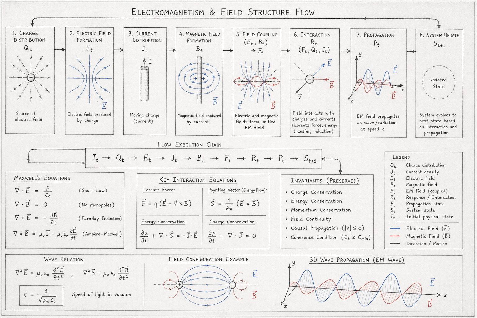
Diagram Overview

This diagram presents electromagnetism as a structured field-execution process. It shows how charge distributions generate electric fields, how moving charge generates magnetic fields, how both fields couple into a unified electromagnetic structure, and how that structure produces interaction, propagation, and system evolution.

The diagram is designed to connect three layers at once:

  • 1. The physical process layer
  • 2. The Flow Algebra execution layer
  • 3. The conventional equation layer

Together, these layers show how electromagnetic behaviour can be read as both classical field physics and executable state transformation.

Telephone:
01377 236594

Upper Flow Sequence

The upper sequence shows the main electromagnetic lifecycle.

The process begins with a charge distribution:

\[ Q_t \]

This charge distribution produces an electric field:

\[ Q_t \rightarrow E_t \]

The diagram then introduces moving charge or current density:

\[ J_t \]

which generates a magnetic field:

\[ J_t \rightarrow B_t \]

The electric and magnetic fields then combine into a unified electromagnetic field:

\[ (E_t, B_t) \rightarrow F_t \]

This coupled field interacts with charges and currents:

\[ (F_t, Q_t, J_t) \rightarrow R_t \]

The interaction may produce force, induction, energy transfer, or radiation.

The electromagnetic field then propagates through space:

\[ F_t \rightarrow P_t \]

Finally, the propagated field and response update the next system state:

\[ (P_t, R_t) \rightarrow S_{t+1} \]

This creates a full causal execution chain from field source to future state.

Flow Execution Chain

The central chain summarises the full process:

It​→Qt​→Et​→Jt​→Bt​→Ft​→Rt​→Pt​→St+1​

This should be read as a continuous state transition.

The initial physical state provides charge and current conditions. These generate electric and magnetic fields. The fields couple, interact, propagate, and update the system.

This means electromagnetism is not shown as a static field diagram, but as an active recursive process.

Telephone:
01377 236594

Maxwell Equation Layer

The lower-left section connects the flow to Maxwell’s equations.

Gauss’s law,

\[ \nabla \cdot \mathbf{E} = \frac{\rho}{\varepsilon_0} \]

links charge density to electric field divergence.

The magnetic continuity equation,

\[ \nabla \cdot \mathbf{B} = 0 \]

states that magnetic field lines do not begin or end at isolated magnetic charges.

Faraday’s induction law,

\[ \nabla \times \mathbf{E} = -\frac{\partial \mathbf{B}}{\partial t} \]

shows that a changing magnetic field generates electric circulation.

The Ampère–Maxwell law,

\[ \nabla \times \mathbf{B} = \mu_0 \mathbf{J} + \mu_0 \varepsilon_0 \frac{\partial \mathbf{E}}{\partial t} \]

shows that current and changing electric fields generate magnetic circulation.

Together, these equations define the classical structure behind the flow sequence.

Interaction Equation Layer

The central lower panel shows the main interaction equations.

The Lorentz force equation,

\[ \mathbf{F} = q \left( \mathbf{E} + \mathbf{v} \times \mathbf{B} \right) \]

describes how electromagnetic fields exert force on moving charge.

The Poynting vector,

\[ \mathbf{S} = \frac{1}{\mu_0} \left( \mathbf{E} \times \mathbf{B} \right) \]

describes electromagnetic energy flow.

The charge conservation equation,

\[ \frac{\partial \rho}{\partial t} + \nabla \cdot \mathbf{J} = 0 \]

ensures that charge is preserved through field evolution.

The energy conservation relation,

\[ \frac{\partial u}{\partial t} + \nabla \cdot \mathbf{S} = -\mathbf{J} \cdot \mathbf{E} \]

shows how electromagnetic energy is transferred between field and matter.

This section makes clear that the diagram is not simply visual. It is tied directly to recognised electromagnetic structure.

Invariants and Stability Conditions

The invariant panel shows the rules that must remain preserved during valid execution.

These include:

\[ Q_{\mathrm{total}}(t+1) = Q_{\mathrm{total}}(t) \]

for charge conservation,

\[ \mathrm{Energy}_{\mathrm{total}}(t+1) = \mathrm{Energy}_{\mathrm{total}}(t) \]

for energy conservation,

and the causal propagation condition:

\[ \lvert v \rvert \leq c \]

meaning electromagnetic influence must remain within the causal speed limit.

The diagram also includes the coherence condition:

\[ C_t \geq C_{\min} \]

This states that the electromagnetic field remains structurally stable only while its internal field relationships remain coherent.

If coherence drops below the threshold, the system may deform, become unstable, or fail to propagate normally.

Wave Propagation Section

The lower wave panel shows electromagnetic propagation.

The electric field and magnetic field oscillate together while travelling through space.

This is represented by the wave equations:

\[ \nabla^2 \mathbf{E} = \mu_0 \varepsilon_0 \frac{\partial^2 \mathbf{E}}{\partial t^2} \]

\[ \nabla^2 \mathbf{B} = \mu_0 \varepsilon_0 \frac{\partial^2 \mathbf{B}}{\partial t^2} \]

The propagation speed is given by:

\[ c = \frac{1}{\sqrt{\mu_0 \varepsilon_0}} \]

This connects the field structure to light-speed electromagnetic wave propagation.

Field Configuration Example

The lower field configuration example shows a local electric and magnetic arrangement between charged bodies.

The electric field lines show directional field organisation between positive and negative charge.

The magnetic structure shows rotational field behaviour associated with dynamic field coupling.

This visual example helps the reader see how the abstract flow relates to real field geometry.

HST Interpretation

process.

Charge distribution represents a boundary coherence imbalance.  Electric field formation represents coherence-gradient organisation.

Current density represents moving coherence structure.

Magnetic field formation represents rotational coherence structure.

Field coupling represents unified coherence geometry.

Propagation represents the transmission of boundary-state information through the field.

The updated state represents recursive coherence reorganisation.

In this reading, electromagnetism is not treated as a separate substance moving through empty space. It is interpreted as a structured expression of evolving boundary coherence.

Scientific Meaning of the Diagram

The diagram shows that electromagnetic behaviour can be understood as a complete executable process:

Source→Field→Coupling→Interaction→
Propagation→Updated State

It combines classical electromagnetic equations with Flow Algebra structure and HST interpretation.

This makes the electromagnetic system readable in three ways:

as a physical field system,

as a mathematical equation system,

and as an executable causal flow.

The central message is that electromagnetic fields are not merely static mathematical descriptions. They are dynamic structures that form, couple, propagate, interact, and recursively update the physical system over time.

Diagram → Flow Mapping Table

Diagram Element Flow Algebra Component Flow Meaning Physical Meaning
Initial Physical State I_t Starting execution state Complete electromagnetic system at time (t)
Charge Distribution Panel Q_t Charge source state Spatial distribution of electric charge
Positive Charge Symbol Q_t > 0 Positive field source Generates outward electric field
Electric Field Lines E_t Electric field state Electric influence surrounding charge
Charge → Electric Field Arrow Q_t → E_t Field generation transformation Charge creates electric field structure
Current Distribution Panel J_t Current state Moving electric charge
Current Arrow (I) J_t Charge motion Electrical current flow
Magnetic Field Rings B_t Magnetic field state Rotational magnetic field generated by current
Current → Magnetic Field Arrow J_t → B_t Magnetic generation transformation Moving charge creates magnetic field
Electric and Magnetic Field Coupling Panel (E_t,B_t) → F_t Field coupling process Unified electromagnetic field formation
Combined Field Structure F_t Electromagnetic field state Coupled electric and magnetic fields
Interaction Panel (F_t,Q_t,J_t) → R_t Field interaction execution Electromagnetic force and induction effects
Charged Particle Symbol Q_t Interaction target Matter responding to field influence
Velocity Vector v Dynamic state variable Motion of charged particle
Electric Force Vector E Field influence Electric force contribution
Magnetic Force Vector B Field influence Magnetic force contribution
Lorentz Interaction Region R_t Response state Force generation and acceleration
Propagation Panel F_t → P_t Field propagation process Electromagnetic wave transmission
Electromagnetic Wave P_t Propagation state Travelling electromagnetic disturbance
Oscillating Electric Field Curve E_t Electric wave component Time-varying electric field
Oscillating Magnetic Field Curve B_t Magnetic wave component Time-varying magnetic field
Wave Travel Direction P_t Propagation vector Direction of energy transport
System Update Panel (P_t,R_t) → S_t+1 State update transformation Future system state generation
Updated State Circle S_t+1 New execution state Physical system after interaction
Flow Execution Chain Box I_t → Q_t → E_t → J_t → B_t → F_t → R_t → P_t → S_t+1 Complete execution path Full electromagnetic lifecycle
Maxwell Equation Panel Governing Rules Constraint layer Mathematical laws governing field behaviour
Gauss Law Equation ∇·E = ρ/ε₀ Electric field constraint Charge generates electric divergence
Magnetic Continuity Equation ∇·B = 0 Magnetic invariant No magnetic monopoles
Faraday Induction Equation ∇×E = -∂B/∂t Coupling rule Magnetic change induces electric field
Ampère-Maxwell Equation ∇×B = μ₀J + μ₀ε₀∂E/∂t Coupling rule Current and electric change induce magnetic field
Lorentz Force Equation Box F = q(E + v×B) Interaction equation Electromagnetic force generation
Poynting Vector Equation S = (1/μ₀)(E×B) Energy flow equation Electromagnetic energy transport
Charge Conservation Equation ∂ρ/∂t + ∇·J = 0 Conservation invariant Total charge preservation
Energy Conservation Equation ∂u/∂t + ∇·S = -J·E Conservation invariant Energy preservation
Invariants Panel C_t Stability layer Physical consistency requirements
Charge Conservation Bullet Q_total(t+1)=Q_total(t) Invariant Charge remains conserved
Energy Conservation Bullet E_total(t+1)=E_total(t) Invariant Energy remains conserved
Momentum Conservation Bullet P_total(t+1)=P_total(t) Invariant Momentum remains conserved
Field Continuity Bullet Continuous Field Evolution Structural invariant Smooth field behaviour
Causal Propagation Bullet v ≤ c Propagation invariant Information cannot exceed light speed
Coherence Condition Bullet C_t ≥ C_min Stability constraint Electromagnetic field remains coherent
Wave Relation Panel P_t Propagation mathematics Electromagnetic wave dynamics
Electric Wave Equation ∇²E = μ₀ε₀∂²E/∂t² Wave propagation rule Electric field wave evolution
Magnetic Wave Equation ∇²B = μ₀ε₀∂²B/∂t² Wave propagation rule Magnetic field wave evolution
Speed of Light Equation c = 1/√(μ₀ε₀) Propagation constant Electromagnetic propagation speed
Field Configuration Example F_t Local field geometry Example electromagnetic structure
Legend Box Symbol Dictionary Mapping reference Interpretation of diagram notation

Complete Diagram Flow

It​→Qt​→Et​→Jt​→Bt​→Ft​→Rt​→Pt​→St+1​

Diagram Logic Summary

Charge→Electric Field→Magnetic Field→Electromagnetic Field→Interaction→Propagation→Updated State

The diagram therefore maps directly onto the Flow Algebra execution chain, showing how charge and current generate fields, how fields couple and interact with matter, how electromagnetic influence propagates through space, and how the resulting interactions recursively update the future state of the system.

Execution Guarantee Statement

Purpose

This Flow Algebra specification defines the complete execution pathway for electromagnetic field formation, interaction, propagation, and system evolution. The flow is constructed such that every valid execution path preserves the fundamental physical invariants governing electromagnetic systems while maintaining causal consistency and structural coherence.

The purpose of this guarantee is to formally define the conditions under which execution remains scientifically valid and physically meaningful.

Execution Guarantee

For every valid system state:

\[ S_t = \left( Q_t,\, E_t,\, B_t,\, F_t,\, P_t,\, R_t,\, C_t \right) \]

the execution sequence

\[ I_t \rightarrow Q_t \rightarrow E_t \rightarrow J_t \rightarrow B_t \rightarrow F_t \rightarrow R_t \rightarrow P_t \rightarrow S_{t+1} \]

is guaranteed to produce a physically valid successor state

\[ S_{t+1} \]

if and only if all invariants and constraints remain satisfied throughout execution.

Deterministic Field Formation Guarantee

Given an identical charge distribution

\[ Q_t \]

and identical boundary conditions, the transformation

\[ Q_t \rightarrow E_t \]

will always generate the same electric field configuration.

Likewise, for a given current density

\[ J_t \]

the transformation

\[ J_t \rightarrow B_t \]

will always generate the same magnetic field configuration.

Therefore:

\[ (Q_t, J_t, \mathrm{Boundary}_t) = \mathrm{constant} \]

implies

\[ (E_t, B_t) = \mathrm{constant} \]

under identical execution conditions.

Electromagnetic Coupling Guarantee

The field coupling transformation

\[ (E_t, B_t) \rightarrow F_t \]

guarantees that electric and magnetic field states combine into a unified electromagnetic field structure.

Provided the input fields remain physically valid,

\[ E_t \neq \emptyset \]

and

\[ B_t \neq \emptyset \]

the resulting electromagnetic state

\[ F_t \]

must exist.

Therefore:

\[ (E_t, B_t) \Rightarrow F_t \]

is guaranteed.

Interaction Guarantee

For any valid electromagnetic field

\[ F_t \]

interacting with charge and current distributions

\[ Q_t \]

and

\[ J_t \]

the response transformation

\[ (F_t, Q_t, J_t) \rightarrow R_t \]

is guaranteed to produce a measurable physical response.

Examples include:

  • Force generation
  • Acceleration
  • Induction
  • Energy transfer
  • Radiation emission
  • Momentum exchange

Thus:

\[ F_t \neq 0 \]

implies

\[ R_t \neq \emptyset \]

whenever an interaction target exists.

Propagation Guarantee

The propagation transformation

\[ F_t \rightarrow P_t \]

guarantees transmission of electromagnetic influence through the surrounding medium.

Propagation remains valid provided:

\[ \mathrm{Medium}_t = \mathrm{valid} \]

and

\[ \lvert v \rvert \leq c \]

where

\[ c = \frac{1}{\sqrt{\mu_0 \varepsilon_0}} \]

is the electromagnetic propagation limit.

No valid execution path permits superluminal propagation.

Telephone:
01377 236594

State Evolution Guarantee

The update transformation

\[ (P_t, R_t) \rightarrow S_{t+1} \]

guarantees that every valid interaction and propagation event contributes to the next system state.

Therefore:

\[ S_t \Rightarrow S_{t+1} \]

whenever all execution constraints remain satisfied.

The system cannot remain static while valid interactions occur.

Conservation Guarantee

Execution preserves the following invariants:

Charge Conservation

\[ Q_{\mathrm{total}}(t+1) = Q_{\mathrm{total}}(t) \]


Energy Conservation

\[ E_{\mathrm{total}}(t+1) = E_{\mathrm{total}}(t) \]


Momentum Conservation

\[ P_{\mathrm{total}}(t+1) = P_{\mathrm{total}}(t) \]


Field Continuity

\[ \mathrm{Field}_{\mathrm{continuous}} = \mathrm{TRUE} \]

except where physically valid boundaries or sources exist.

These invariants remain true for every valid execution cycle.

Coherence Guarantee

The electromagnetic field remains stable only when:

\[ C_t \geq C_{\min} \]

where:

\[ C_t \]

represents field coherence.

Under this condition:

\[ \mathrm{Execution}(S_t) = \mathrm{STABLE} \]

and all field transformations remain physically meaningful.

Failure Guarantee

Execution is guaranteed to terminate as invalid whenever any of the following occur:

Undefined Charge Source

\[ Q_t = \emptyset \]


Invalid Boundary Conditions

\[ \mathrm{Boundary}_t = \mathrm{invalid} \]


Coherence Collapse

\[ C_t < C_{\min} \]


Causality Violation

\[ \lvert v \rvert > c \]

Under these conditions:

\[ \mathrm{Execution}(S_t) = \mathrm{FAIL\_OR\_DEFORM} \]

and the resulting state is considered physically non-valid.

Recursive Execution Guarantee

The electromagnetic lifecycle is recursively executable:

\[ S_t \rightarrow S_{t+1} \rightarrow S_{t+2} \rightarrow S_{t+3} \rightarrow \cdots \]

Each state becomes the input to the next execution cycle.

Provided all invariants remain satisfied, execution may continue indefinitely without logical contradiction.

Telephone:
01377 236594

HST Execution Guarantee

Within the Holographic Space-Time interpretation, charge distributions, currents, electric fields, magnetic fields, and electromagnetic waves are treated as evolving boundary-coherence structures.

The flow guarantees that:

Coherencet​→Fieldt​→Interactiont​→Propagationt​→Coherencet+1​

remains structurally consistent whenever coherence remains above the minimum stability threshold.

Thus, electromagnetic phenomena emerge as recursively stable coherence transformations rather than isolated field events.

Formal Guarantee Statement

\[ (Q_t \neq \emptyset) \;\wedge\; (\mathrm{Boundary}_t = \mathrm{valid}) \;\wedge\; (C_t \geq C_{\min}) \;\wedge\; (\lvert v \rvert \leq c) \]

⟹

\[ \mathrm{Execution}(S_t) = \mathrm{STABLE} \]

⟹

\[ \exists S_{t+1} \]

⟹

\[ S_t \rightarrow S_{t+1} \]

with preservation of charge, energy, momentum, field continuity, and causal propagation throughout the complete electromagnetic execution cycle.

Section Chapters
Kireth Research
38 Thorndale Croft, Wetwang, Driffield
East Riding of Yorkshire YO25 9XZ
Telephone: 01377 236594
Designed By