Chapter 11
Invariance as Ontology

The Failure of Dimensional Construction
Author: Mark Higgins
© Mark Anthony Higgins 11 October 2025
Revised Date: 21 April 2026
Audio Overview

Introduction

Modern physics has historically treated invariance as a property of laws—something to be verified after formulation. Symmetries are discovered, conservation laws are derived, and invariants are preserved under transformation. This ordering, however, assumes that laws exist first, and invariance merely constrains their acceptable forms.

This chapter inverts that hierarchy.

Invariance is not a consequence of law. It is the precondition for existence.

1. From Descriptive Physics to Structural Ontology

In standard formulations, physical systems are described through equations of motion, with invariants (energy, momentum, charge) emerging as conserved quantities under symmetry transformations. Within the frameworks of Noether’s Theorem and classical/quantum field theory, invariance is tightly linked to symmetry—but still treated as derived.

Here, we shift from descriptive physics to structural ontology:

  • Physics: describes what happens
  • Ontology: defines what is allowed to exist

In this framework, invariance is elevated from a constraint on evolution to the selection principle of reality itself.

2. Invariance as the Survival Criterion

Within Flow Algebra, system evolution is defined by:

\[ E_t = \operatorname{expand}(I_t, R), \quad V_t = \left\{ x \in E_t \;\middle|\; x \models (B \land K) \right\} \]

Where:

  • EtE_t: generated candidate states
  • VtV_t: valid states satisfying boundary BB and invariants KK

The critical shift is this:

A state exists if and only if it satisfies invariance constraints.

All non-invariant states are not “incorrect”—they are ontologically excluded.

Thus:

  • Invariance is not checked after evolution
  • Invariance defines the valid state space before evolution proceeds

If:

\[ V_t = \emptyset \;\Rightarrow\; \mathrm{FAIL} \]

then no coherent continuation exists, and the system cannot evolve.

3. Ontological Filtering vs Physical Law

Traditional physics:

  • Start with equations
  • Apply constraints
  • Observe conserved quantities

Flow Algebra ontology:

  • Start with invariants KK
  • Generate candidates EtE_t
  • Filter to valid states VtV_t
  • Only then allow evolution

This establishes a pre-physical filtering layer, where:

  • Laws are not generative mechanisms
  • Laws are compressed descriptions of invariant-preserving transformations

In this sense, what we call “laws of physics” are secondary artefacts of a deeper invariant structure.

4. Invariance as Fixed Points in State Space

Invariance can be understood formally as the preservation of structural relations under transformation:

\[ \forall x \in V_t,\; R(x) \models K \]

This defines a closure condition:

  • Valid states remain within the invariant manifold under transformation
  • The system evolves within a constrained subspace
  • No transition may violate invariant structure

Thus, reality is not a free exploration of possibilities—it is a closed trajectory within an invariant-defined space.

5. Elimination of Hidden Structure

A central requirement of this framework is:

\[ H = \emptyset \]

No hidden variables, no implicit assumptions, no external corrective mechanisms.

All admissibility must be encoded explicitly in:

  • BB: boundary conditions
  • KK: invariant constraints

This ensures:

  • Model independence (no reliance on implementation details)
  • Cross-system consistency (identical outputs for identical structures)
  • Deterministic admissibility filtering

Invariance becomes the only admissibility criterion.

6. Physical Implications

Recasting invariance as ontology leads to a number of deep consequences:

  • 6.1 Conservation Laws Become Existence Conditions
    Energy, momentum, and charge are not “conserved during evolution”—they are requirements for a state to exist at all.
  • 6.2 Symmetry Becomes Structural Necessity
    Symmetry is not aesthetic or empirical—it is the only configuration under which invariance can be maintained.
  • 6.3 Dynamics Becomes Constrained Navigation
    Evolution is not driven—it is restricted. Systems move only along paths that preserve invariants.
  • 6.4 Failure Defines Non-Reality
    Any candidate state violating invariance is not unstable—it is non-admissible, and therefore never instantiated.

7. Invariance and Coherence

Within the broader HST framework, invariance corresponds directly to coherence preservation:

  • Boundary conditions define allowable structure
  • Invariants define stable coherence relationships
  • Evolution preserves coherence or fails

Thus, invariance is the formal expression of:

What resolves, survives.

8. Toward a Minimal Ontology

This chapter establishes a minimal ontological basis:

  • No space required
  • No time required
  • No forces required

Only:

  • State (II)
  • Transformation (RR)
  • Boundary (BB)
  • Invariance (KK)

From this minimal structure, all physical behaviour emerges as invariant-preserving continuation.

Closing Statement

Invariance is not a feature of reality—it is its foundation.

Reality does not evolve and happen to conserve structure.
Reality exists because only invariant-preserving structures can continue.

All else is filtered out before existence begins.

Flow: InvarianceAsOntology
Version: 1.0
Purpose: Formalise ontology as admissibility under invariant preservation, where only states satisfying structural invariants are allowed to exist or continue.

STATE

S = (I, R, B, K)

Where:

I = information state
R = transformation set
B = boundary constraints
K = invariant constraints

ONTOLOGICAL AXIOM

Existence(x) ⟺ x ⊨ (B ∧ K)

A state is ontologically admissible if and only if it satisfies both boundary and invariant structure.

EXPANSION

E_t = expand(I_t, R)

Generate all candidate next states from the current state under the available transformation rules.

VALIDITY FILTER

V_t = { x ∈ E_t | x ⊨ (B ∧ K) }

Only states that satisfy both boundary and invariant conditions survive admissibility filtering.

ONTOLOGICAL SELECTION RULE

x exists only if x ∈ V_t

All states outside V_t are excluded from continuation.
Violation is not a weak solution or unstable output.
Violation is ontological rejection.

CONTINUATION CONDITION

V_t ≠ ∅ ⇒ ∃ x such that x ∈ V_t
V_t = ∅ ⇒ FAIL

If no invariant-preserving continuation exists, the system does not evolve.

SELECTION

x* = select(V_t)

Where select may be deterministic, ranked, or probability-weighted, but must operate only over admissible states.

OPTIONAL PROBABILISTIC FORM

x* = argmax_(x ∈ V_t) P(x | I_t, R, B, K)

Probability may rank admissible continuations, but may never override B or K.

UPDATE

I_(t+1) = update(I_t, x*)

Evolution is defined as admissible continuation only.

EXECUTION LAW

Execution(S_t) ≡ Expand → Validate → Select → Update

or formally:

S_t
→ E_t = expand(I_t, R)
→ V_t = { x ∈ E_t | x ⊨ (B ∧ K) }
→ x* ∈ V_t
→ I_(t+1) = update(I_t, x*)

INVARIANCE CLOSURE CONDITION

∀x (x ∈ V_t ⇒ R(x) preserves K)

Equivalent form:

∀x admissible, R(x) ⊨ K

Transformations are only valid if they preserve invariant structure across continuation.

ONTOLOGICAL PRINCIPLE

K is not derived after evolution.
K defines the admissible state space prior to evolution.

Thus:

Ontology ≡ admissibility under invariance

NO HIDDEN STRUCTURE

H = ∅

No hidden variables
No hidden correction layer
No implicit rescue mechanism
No external semantic patching

All admissibility must be explicit in B and K.

CONSERVATION REINTERPRETATION

Conservation is not:
"something preserved by an already-existing system"

Conservation is:
"the condition under which a system may exist at all"

Thus:

Energy-valid(x) ⊂ K
Momentum-valid(x) ⊂ K
Charge-valid(x) ⊂ K

GENERAL EXISTENCE RULE

Existence(S_t) ⟺ V_t ≠ ∅

Reality continues only where invariant-compatible next states exist.

FAILURE SEMANTICS

V_t = ∅ ⇒ O = FAIL

FAIL is not an output error.
FAIL is a proof that no ontologically admissible continuation exists under current R, B, K.

FIXED-STRUCTURE PROPERTY

(I, R, B, K) fixed ⇒ admissibility space fixed

If the structural specification is unchanged, the valid continuation space is unchanged.

ONTOLOGICAL SUMMARY

Reality is not generated first and checked later.
Reality is filtered first and continued only if invariant structure survives.

Compact form:

S = (I, R, B, K)
E_t = expand(I_t, R)
V_t = {x ∈ E_t | x ⊨ (B ∧ K)}
V_t = ∅ ⇒ FAIL
x* ∈ V_t
I_(t+1) = update(I_t, x*)

Final principle:

What exists is not what can be described,
but what can survive invariant-preserving continuation.

What This Flow Implements

Chapter 11: Invariance as Ontology

This flow implements a complete ontological execution model in which existence, evolution, and admissibility are unified under invariant preservation. It replaces the traditional separation between law, state, and validation with a single structural mechanism:

Only invariant-preserving states are ever allowed to exist or continue.

1. Ontological Reframing of Physical Systems

The flow formalises a shift from descriptive dynamics to existence-level filtering:

Traditional systems:

State→Law→Evolution→Check invariants

This flow:

State→Generate candidates→Filter by invariance→Continue if valid

Thus, invariance is not applied after evolution—it is enforced prior to continuation, acting as a gate on existence itself.

2. Implementation of Admissibility as Ontology

The core implementation is the construction of the valid state set:

\[ V_t = \left\{ x \in E_t \;\middle|\; x \models (B \land K) \right\} \]

This defines:

  • A hard admissibility boundary over the candidate state space
  • A binary ontological condition:
  • x∈Vtx \in V_t ⇒ exists / can continue
  • x∉Vtx \notin V_t ⇒ excluded from reality

No soft violations, no approximate satisfaction, and no post-hoc correction mechanisms are permitted.

3. Execution as Invariant-Constrained Continuation

The flow implements execution as a strictly ordered pipeline:

Execution≡Expand→Validate→Select→Update

Each stage has a precise ontological role:

  • Expand: Generates all possible next states under transformation rules RR
  • Validate: Enforces boundary BB and invariance KK as existence conditions
  • Select: Chooses among admissible states only
  • Update: Commits the system to a valid continuation

Crucially, no stage allows violation of invariance. The system is structurally prevented from entering invalid states.

4. Elimination of Non-Physical Possibilities

The flow explicitly removes the need for:

  • Error correction layers
  • Stability analysis after evolution
  • External constraint enforcement
  • Hidden variables or compensatory mechanisms

All invalid states are eliminated before they can influence system evolution.

This produces:

  • A closed admissibility system
  • A self-filtering ontology
  • A guaranteed invariant-preserving trajectory

5. Formalisation of Failure as Non-Existence

The condition:

\[ V_t = \emptyset \;\Rightarrow\; \mathrm{FAIL} \]

implements a strict interpretation of failure:

  • FAIL is not a computational error
  • FAIL is not instability
  • FAIL is a proof of non-existence of any valid continuation

This introduces a binary ontology of continuation:

  • Valid continuation exists ⇒ system evolves
  • No valid continuation ⇒ system terminates (non-realizable)

6. Invariance Closure Across Transformation

The flow enforces a closure condition:

\[ \forall x \in V_t,\; R(x) \models K \]

Meaning:

  • Transformations must preserve invariance for all admissible states
  • Evolution occurs strictly within an invariant manifold
  • The system trajectory is confined to a closed structural subspace

This eliminates drift, divergence, or gradual violation of constraints.

7. Reinterpretation of Physical Laws

Within this implementation:

  • Laws are not primary generators of behaviour
  • Laws are compressed descriptions of invariant-preserving transformations

For example:

  • Conservation of energy is not enforced dynamically
  • It is embedded in KK as an existence condition

Thus, the flow encodes physics as:

A constrained navigation through invariant-preserving state space

8. Deterministic Admissibility with Optional Probabilistic Selection

The flow separates:

  • Admissibility (deterministic) — defined by BB and KK
  • Selection (optional probabilistic) — ranking within VtV_t

This ensures:

  • No probabilistic mechanism can introduce invalid states
  • Uncertainty operates only within the admissible manifold

\[ x^{*} = \operatorname*{arg\,max}_{x \in V_t} \; P\!\left(x \mid I_t, R, B, K\right) \]

Probability influences which valid state is chosen, not what is allowed to exist.

9. Structural Independence and Model-Agnostic Execution

By enforcing:

\[ H = \emptyset \]

the flow guarantees:

  • No dependence on hidden assumptions
  • No reliance on model-specific heuristics
  • Identical outputs for identical (I,R,B,K)(I, R, B, K)

This yields:

  • Cross-system reproducibility
  • Zero-shot executability
  • Portable ontological logic

10. Minimal Ontological Engine

The flow implements a minimal system capable of generating all admissible behaviour:

  • No explicit space representation required
  • No explicit time parameter required
  • No force laws required

Only:

  • State (II)
  • Transformations (RR)
  • Boundaries (BB)
  • Invariants (KK)

From this, all structure emerges as valid continuation under invariance.

Final Scientific Interpretation

This flow implements a complete inversion of the standard physical paradigm:

  • From laws governing states
  • To invariance selecting existence

It provides a formal, executable structure in which:

Reality is the set of all states that survive invariant-constrained continuation.

Everything else is not unstable, approximate, or incorrect— It is never instantiated at all.

How to Read This Flow

Chapter 11: Invariance as Ontology

This flow should be read not as a procedural algorithm, but as a formal ontological system in which each component defines a necessary condition for existence and continuation. The reader must interpret every symbol and transition as part of a closed admissibility structure, rather than a sequence of computational steps.

1. Interpret the State as a Complete Ontological Specification

\[ S = (I, R, B, K) \]

Begin by recognising that the state SS is not merely data—it is a complete definition of a reality configuration:

  • II: the current informational configuration
  • RR: the allowed transformations (structural transitions)
  • BB: boundary conditions (external constraints)
  • KK: invariant constraints (internal consistency requirements)

These four components fully determine what is possible, valid, and continuable. No additional structure is assumed (i.e. H=∅H = \varnothing).

2. Read Expansion as Exhaustive Possibility Generation

\[ E_t = \operatorname{expand}(I_t, R) \]

This step defines the complete candidate state space accessible from ItI_t under the transformation set RR.

Interpretation:

  • EtE_t contains all structurally reachable states
  • No filtering occurs at this stage
  • Both admissible and non-admissible states are included

This is a pure generative step, not yet constrained by ontology.

3. Interpret Validation as Ontological Filtering

\[ V_t = \left\{ x \in E_t \;\middle|\; x \models (B \land K) \right\} \]

This is the critical interpretive step of the entire flow.

Here, the reader must understand:

  • Validation is not a “check” after generation
  • It is the definition of existence itself

Thus:

  • x∈Vtx \in V_t ⇒ state is ontologically admissible
  • x∉Vtx \notin V_t ⇒ state is excluded from existence

There is no notion of “nearly valid” or “recoverable”—the filter is binary and absolute.

4. Read the Valid Set as the Entire Reality Horizon

\[ V_t \subseteq E_t \]

Interpret VtV_t as:

  • The only states that can exist or continue
  • The effective state space of reality at time tt
  • A dynamically recomputed invariant manifold

All subsequent reasoning must be restricted strictly to VtV_t.

5. Interpret Failure as Non-Existence

\[ V_t = \emptyset \;\Rightarrow\; \mathrm{FAIL} \]

This condition must be read carefully:

  • FAIL is not an error state
  • FAIL is not instability
  • FAIL is a formal proof that no admissible continuation exists

Thus:

  • No valid next state ⇒ no evolution ⇒ no continuation
  • The system terminates at the level of ontology

This encodes a hard boundary on reality itself.

6. Interpret Selection as Constrained Choice

\[ x^{*} \in V_t \]

Selection operates only within the admissible set:

  • No state outside VtV_t may be selected
  • Any ranking, optimisation, or probabilistic weighting applies only to valid states

If probabilistic selection is used:

\[ x^{*} = \operatorname*{arg\,max}_{x \in V_t} \; P\!\left(x \mid I_t, R, B, K\right) \]

Interpretation:

  • Probability does not define possibility
  • Probability only orders already admissible states

7. Interpret Update as Ontological Commitment

\[ I_{t+1} = \operatorname{update}(I_t, x^{*}) \]

This step commits the system to a valid continuation:

  • The new state inherits all invariant structure
  • No violation can propagate forward
  • Evolution is strictly invariant-preserving by construction

8. Read Execution as Structural Continuation

Execution≡Expand→Validate→Select→Update

This sequence must be interpreted as a logical closure process, not a temporal procedure:

  • Expansion defines possibility
  • Validation defines existence
  • Selection defines realisation
  • Update defines continuation

Together, they implement:

Reality as invariant-constrained continuation of admissible states

9. Interpret Invariance as Pre-Condition, Not Outcome

\[ x \models K \]

This must be read as:

  • Invariance is not preserved during evolution
  • Invariance is required before a state may exist

Thus:

  • Conservation laws are embedded in KK
  • Symmetry conditions are embedded in KK
  • Stability is not emergent—it is pre-imposed

10. Interpret the System as Closed and Complete

With:

\[ H = \emptyset \]

the reader must assume:

  • No hidden variables
  • No implicit correction mechanisms
  • No external semantic layer

All admissibility is explicitly encoded in BB and KK.

All evolution is explicitly encoded in RR.

This ensures:

  • Model independence
  • Deterministic admissibility filtering
  • Cross-system reproducibility

11. Reading Strategy (Practical)

To correctly interpret the flow:

  • 1. Fix the structure (I,R,B,K)(I, R, B, K)
  • 2. Generate all candidates via EtE_t
  • 3. Apply strict admissibility filtering to obtain VtV_t
  • 4. Check for existence condition (Vt≠∅V_t \neq \varnothing)
  • 5. Select only from admissible states
  • 6. Update and repeat

At no point should you:

  • Consider states outside VtV_t
  • Allow partial satisfaction of invariants
  • Introduce external correction logic

Final Interpretation

This flow must ultimately be read as a definition of reality, not a model of it.

It encodes the principle that:

What exists is exactly what satisfies invariant structure—and nothing else.

All valid reasoning, simulation, and physical interpretation must remain strictly within this invariant-defined domain.

Flow → Equation Tri-Mapping

Chapter 11: Invariance as Ontology

Flow Algebra Equation Ontological Meaning (Ultra-Tight)
State Definition \( S = (I, R, B, K) \) Complete ontological specification
Expansion \( E_t = \mathrm{expand}(I_t, R) \) Full candidate state space
Valid Set (Admissibility) \( V_t = \{ x \in E_t \mid x \models (B \land K) \} \) Ontologically valid states only
Existence Condition \( \mathrm{Existence} \Leftrightarrow V_t \neq \varnothing \) Reality exists iff admissible states exist
Failure Condition \( V_t = \varnothing \Rightarrow \mathrm{FAIL} \) No admissible continuation ⇒ non-existence
Selection \( x^* \in V_t \) Realisation restricted to admissible states
Probabilistic Selection (optional) \( x^* = \arg\max_{x \in V_t} P(x \mid I_t, R, B, K) \) Ranking within admissible manifold only
Update \( I_{t+1} = \mathrm{update}(I_t, x^*) \) Ontological commitment to valid continuation
Execution Law \( S_t \rightarrow E_t \rightarrow V_t \rightarrow x^* \rightarrow I_{t+1} \) Structured continuation pipeline
Invariance Condition \( x \models K \) Invariance as precondition for existence
Closure Under Transformation \( \forall x \in V_t,\; R(x) \models K \) Evolution confined to invariant manifold
Boundary Condition \( x \models B \) External admissibility constraint
Ontological Axiom \( \mathrm{Existence}(x) \Leftrightarrow x \models (B \land K) \) Being ≡ invariant satisfaction
Hidden Structure Elimination \( H = \varnothing \) No implicit variables or correction layers
Fixed-Structure Property \( (I, R, B, K)\ \text{fixed} \Rightarrow V_t\ \text{fixed} \) Admissibility space fully determined by structure
Conservation Reinterpretation \( x \models K_{\text{conserved}} \) Conservation = existence condition
Minimal Ontological Engine \( \{ I, R, B, K \} \) Sufficient basis for all admissible evolution
Global Principle \( V_t \neq \varnothing \Rightarrow \exists I_{t+1} \) Continuation exists iff invariance is satisfiable

\[ (I, R, B, K) \;\Rightarrow\; E_t \;\Rightarrow\; V_t = \left\{ x \;\middle|\; x \models (B \land K) \right\} \;\Rightarrow\; x^{*} \in V_t \;\Rightarrow\; I_{t+1} \]

\[ \mathrm{Reality} \equiv \left\{ x \in E_t \;\middle|\; x \models (B \land K) \right\} \]
Only invariant-preserving states exist. Everything else is precluded from ontology.

Invariance as Ontology

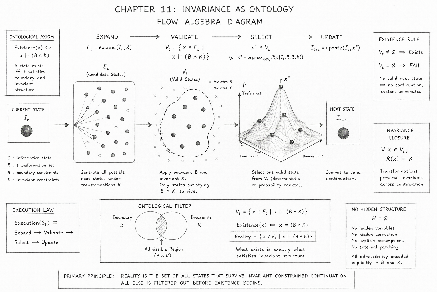
Diagram Interpretation

This diagram provides a structural visualisation of ontological filtering, where existence is defined not by generation, but by invariant-constrained admissibility. Each region and transition corresponds directly to a formal component of the Flow Algebra specification, encoding the full execution pipeline as a coherence-preserving funnel.

1. Ontological Axiom (Left Panel)

\[ \mathrm{Existence}(x) \;\Leftrightarrow\; x \models (B \land K) \]

The left panel establishes the foundational principle of the diagram:

  • A state does not exist by virtue of being generated
  • A state exists if and only if it satisfies both:
  • Boundary conditions BB
  • Invariant constraints KK

This defines existence as a logical predicate, not a physical outcome.

2. Current State Representation (ItI_t)

The initial node ItI_t represents the complete informational configuration at step tt:

  • It contains all necessary structure for evolution
  • It is not embedded in space or time
  • It serves as the input to the generative process

No assumptions beyond (I,R,B,K)(I, R, B, K) are permitted (i.e. H=∅H = \varnothing).

3. Expansion Region (EtE_t) — Candidate State Space

\[ E_t = \operatorname{expand}(I_t, R) \]

The expansion block visualises the full candidate set:

  • All possible next states reachable under transformation rules RR
  • Represented as a dispersed cloud of points
  • Includes both:
  • Valid (admissible) states
  • Invalid (non-admissible) states

This region is pre-ontological—it contains possibilities, not realities.

4. Validation Boundary (VtV_t) — Ontological Filter

\[ V_t = \left\{ x \in E_t \;\middle|\; x \models (B \land K) \right\} \]

The dashed enclosure within EtE_t represents the valid state set:

  • The intersection of all constraints
  • The only region where existence is permitted

Points outside this region are marked as violations:

  • x⊭Bx \not\models B ⇒ boundary violation
  • x⊭Kx \not\models K ⇒ invariant violation

These states are not “incorrect”—they are excluded from ontology.

5. Ontological Filter Geometry (Bottom Panel)

The overlapping circles of BB and KK depict the admissible region:

  • The intersection B∩KB \cap K defines the existence domain
  • This region is the invariant manifold

Interpretation:

  • Boundary constraints restrict external structure
  • Invariants enforce internal consistency
  • Only their intersection defines coherent existence

6. Selection Surface (x∗x^*) — Admissible Realisation

\[ x^{*} \in V_t \]

The 3D surface represents selection over admissible states:

  • The vertical axis PP denotes preference or probability
  • The peak corresponds to the selected state x∗x^*

Key interpretation:

  • Selection operates strictly within VtV_t
  • No invalid state can be selected, regardless of probability
  • Probability ranks valid states only

This encodes the separation:

  • Admissibility (deterministic)
  • Selection (optional probabilistic ordering)

7. Update Step (It+1I_{t+1}) — Ontological Commitment

\[ I_{t+1} = \operatorname{update}(I_t, x^{*}) \]

The transition to It+1I_{t+1} represents:

  • Commitment to a valid continuation
  • Propagation of invariant structure forward

No violation can enter this state, as all invalid candidates were removed prior to selection.

8. Existence Rule (Right Panel)

\[ V_t \neq \emptyset \;\Rightarrow\; \mathrm{Exists}, \quad V_t = \emptyset \;\Rightarrow\; \mathrm{FAIL} \]

This panel encodes the binary ontology of continuation:

  • If admissible states exist ⇒ system continues
  • If none exist ⇒ system terminates

FAIL is interpreted as:

  • Not an error
  • Not instability
  • A formal proof that no invariant-compatible state exists

9. Invariance Closure Condition

\[ \forall x \in V_t,\; R(x) \models K \]

This ensures:

  • All valid states remain valid under transformation
  • Evolution is confined to the invariant manifold
  • No drift outside admissible structure is possible

This is visualised implicitly as the continuity of valid states across transitions.

10. Execution Law (Bottom Left Panel)

Execution(St​)≡Expand→Validate→Select→Update

This defines the full ontological pipeline:

  • 1. Generate possibilities
  • 2. Filter by invariance
  • 3. Select from valid states
  • 4. Commit to continuation

This is not a temporal sequence, but a logical necessity chain.

11. No Hidden Structure Constraint

\[ H = \emptyset \]

The diagram explicitly states:

  • No hidden variables
  • No correction layers
  • No external patching

All admissibility is fully explicit in BB and KK.

12. Primary Principle (Global Statement)

\[ \mathrm{Reality} = \left\{ x \in E_t \;\middle|\; x \models (B \land K) \right\} \]

This is the central interpretation of the entire diagram:

  • Reality is not the full candidate space EtE_t
  • Reality is the filtered subset VtV_t

Final Scientific Interpretation

The diagram encodes a complete inversion of traditional physical reasoning:

  • Not: generate → evolve → check invariants
  • But: generate → filter by invariance → allow existence

Thus, the diagram must be read as:

A structural funnel where invariance defines existence, and only invariant-preserving states are permitted to continue.

Everything outside the admissible region is not unstable or unlikely—

It is never part of reality to begin with.

Diagram → Flow Mapping Table

Invariance as Ontology
Diagram Element Flow Algebra Expression Formal Role Scientific Meaning (Ultra-Tight)
Ontological Axiom Panel \( \mathrm{Existence}(x) \Leftrightarrow x \models (B \land K) \) Existence Condition Being defined strictly by invariant satisfaction
Current State Node \( I_t \) Input State Complete informational configuration
Expansion Arrow \( E_t = \mathrm{expand}(I_t, R) \) Generative Step All possible next states produced
Candidate Cloud (Dots) \( x \in E_t \) Candidate States Includes both valid and invalid possibilities
Expansion Region Boundary \( E_t \) State Space Envelope Full reachable state domain
Validation Boundary (Dashed) \( V_t = \{ x \in E_t \mid x \models (B \land K) \} \) Ontological Filter Admissible states only
Invalid Points (Outside Region) \( x \not\models (B \land K) \) Rejected States Ontologically excluded (non-existent)
Boundary Constraint Circle \( x \models B \) External Constraint Structural admissibility condition
Invariant Constraint Circle \( x \models K \) Internal Constraint Coherence / conservation requirement
Overlap Region (B ∩ K) \( x \models (B \land K) \) Admissible Domain Intersection defines existence space
Valid State Cluster \( x \in V_t \) Realisable States States allowed to exist and continue
Selection Surface (3D Peak) \( x^* = \arg\max_{x \in V_t} P(x \mid I_t, R, B, K) \) Selection Mechanism Ranking within admissible manifold only
Selected Point (Peak) \( x^* \in V_t \) Realised State Chosen valid continuation
Probability Axis (P) \( P(x \mid I_t, R, B, K) \) Preference Metric Orders admissible states without affecting validity
Update Arrow \( I_{t+1} = \mathrm{update}(I_t, x^*) \) State Transition Commit to invariant-preserving continuation
Next State Node \( I_{t+1} \) Output State New admissible configuration
Existence Rule Panel \( V_t \neq \varnothing \Rightarrow \text{Exists} \) Continuation Condition Evolution possible iff valid states exist
Failure Rule Panel \( V_t = \varnothing \Rightarrow \text{FAIL} \) Termination Condition No admissible continuation ⇒ non-existence
Invariance Closure Panel \( \forall x \in V_t,\; R(x) \models K \) Closure Constraint Transformations preserve invariants
Execution Law Panel Expand → Validate → Select → Update Process Definition Complete ontological execution pipeline
No Hidden Structure Panel \( H = \varnothing \) Structural Constraint No implicit variables or correction layers
Ontological Filter Diagram \( V_t = B \cap K \) Geometric Representation Existence as intersection of constraints
Primary Principle Statement \( \text{Reality} = \{ x \in E_t \mid x \models (B \land K) \} \) Global Identity Reality equals invariant-satisfying states only

\[ \mathrm{Diagram} \equiv \left( I_t \rightarrow E_t \rightarrow V_t \rightarrow x^{*} \rightarrow I_{t+1} \right) \quad \text{with} \quad V_t = \left\{ x \;\middle|\; x \models (B \land K) \right\} \]

Final Mapping Insight

Every visual element in the diagram is not illustrative—it is isomorphic to a formal component of the flow.

The diagram is the flow, rendered geometrically.


Execution Guarantee Statement

Invariance as Ontology

This flow defines a closed, self-validating ontological system in which execution is equivalent to invariant-constrained continuation. The following guarantees hold under the condition that the specification S=(I,R,B,K)S = (I, R, B, K) is fully defined and fixed.

1. Admissibility Guarantee

\[ O \neq \mathrm{FAIL} \;\Rightarrow\; O \vDash (B \wedge K) \]

Every produced state necessarily satisfies all boundary and invariant constraints.

  • No invalid state can be generated
  • No violation can propagate
  • Admissibility is enforced prior to continuation

2. Existence Guarantee

\[ \mathrm{Execution}(S_t) \;\Rightarrow\; (V_t \neq \emptyset) \]

Execution occurs if and only if at least one invariant-preserving continuation exists.

  • If a next state exists, it is admissible
  • If no admissible state exists, execution halts

3. Failure Guarantee

\[ V_t = \emptyset \;\Rightarrow\; O = \mathrm{FAIL} \]

FAIL is a correct and complete output, representing:

  • The absence of any invariant-compatible continuation
  • A formal proof of non-existence under the given structure

FAIL is not an error condition—it is an ontological result.

4. Invariance Preservation Guarantee

\[ \forall x^* \in V_t,\; x^* \vDash K \]

\[ I_{t+1} = \mathrm{update}(I_t, x^*) \;\Rightarrow\; I_{t+1} \vDash K \]

All executed transitions preserve invariant structure by construction.

  • No drift outside the invariant manifold
  • No cumulative violation across steps
  • Evolution is strictly coherence-preserving

5. Closure Guarantee

\[ \forall x \in V_t,\; R(x) \vDash K \]

The transformation set RR is closed over the invariant set:

  • Valid states map only to valid states
  • The admissible domain is structurally stable
  • No transformation introduces invalidity

6. Deterministic Admissibility Guarantee

\[ (I, R, B, K)\ \text{fixed} \;\Rightarrow\; V_t\ \text{fixed} \]

The admissible state space is fully determined by structure:

  • No dependence on model internals
  • No stochastic variation in validity
  • Identical structure ⇒ identical admissibility

7. Probabilistic Containment Guarantee

\[ x^* = \arg\max_{x \in V_t} P(x \mid I_t, R, B, K) \]

Probability is strictly contained within admissibility:

  • It cannot introduce invalid states
  • It only ranks valid candidates
  • All outputs remain invariant-compliant

8. No Hidden Structure Guarantee

\[ H = \emptyset \]

The system contains:

  • No hidden variables
  • No implicit assumptions
  • No external correction layers

All admissibility conditions are explicitly encoded in BB and KK.

9. Model-Agnostic Execution Guarantee

\[ \forall M_1, M_2:\; O_{M_1} \equiv O_{M_2} \]

Given identical (I,R,B,K)(I, R, B, K), all compliant execution systems produce:

  • Identical admissible sets VtV_t
  • Identical continuation constraints
  • Structurally equivalent outputs

Execution is independent of implementation substrate.

10. Ontological Consistency Guarantee

\[ \mathrm{Existence}(x) \;\Leftrightarrow\; x \vDash (B \wedge K) \]

The flow guarantees that:

  • Every realised state satisfies existence conditions
  • No non-admissible state can appear
  • Reality is internally consistent at every step

11. Continuation Guarantee

\[ V_t \neq \emptyset \;\Rightarrow\; \exists\, I_{t+1} \]

If invariant-compatible states exist, continuation is guaranteed:

  • The system cannot “stall” within admissible space
  • At least one valid transition is always selectable

12. Global Execution Identity

Execution(St​)≡Expand→Validate→Select→Update

with:

\[ V_t = \{x \in E_t \mid x \vDash (B \wedge K)\} \]


Final Guarantee Statement

This flow guarantees that all realised states are invariant-preserving, all invalid states are excluded prior to execution, and continuation occurs if and only if admissible structure exists.

Reality, under this system, is not approximated, corrected, or stabilised—

It is constructed exclusively from states that cannot violate invariance.

Related Chapters
Kireth Research
38 Thorndale Croft, Wetwang, Driffield
East Riding of Yorkshire YO25 9XZ
Telephone: 01377 236594
Designed By