Chapter 39
Wave Propagation as Boundary Transfer

This flow implements the Holographic Space-Time (HST) interpretation of wave propagation, in which waves are not treated as physical objects moving through an independent space, but as recursive transfers of coherence information between neighbouring boundary states.

The flow formalises the complete causal chain by which a local disturbance generates a coherence gradient, produces directional transfer currents, updates adjacent boundaries, and ultimately creates the observable phenomenon identified as wave motion.

Rather than modelling waves as oscillating substances travelling through a medium, the flow models propagation as a sequence of information-preserving boundary updates. Apparent motion emerges because neighbouring regions continuously inherit and transmit coherence structures from one another.

The implementation therefore transforms wave mechanics into a problem of recursive information transfer across a dynamic coherence network.

The central hypothesis implemented by this flow is:

In conventional physics, propagation is often described as:

Wave Source→Medium→Wave Motion

In HST, the process becomes:

\[ B_t \rightarrow C_t \rightarrow \nabla C_t \rightarrow J_C \rightarrow B_{t+1} \]

where:

The observable wavefront emerges from repeated execution of this transfer cycle.

The first stage implemented by the flow is disturbance detection.

A wave begins when local coherence is altered.

The system converts incoming information into a modified boundary configuration:

\[ I_t \rightarrow B_t \]

The resulting coherence map is then generated:

\[ C_t = \mathrm{CoherenceMap}(B_t) \]

The flow continuously evaluates the spatial coherence structure and calculates gradients:

\[ G_t = \nabla C_t \]

A non-zero gradient indicates that neighbouring regions possess different coherence states.

This difference becomes the driving force for propagation.

The flow implements wave motion as a direct consequence of coherence imbalance.

Whenever:

\[ \nabla C_t \neq 0 \]

the system identifies an information-pressure differential.

This is analogous to:

Within HST the quantity being redistributed is coherence itself.

The gradient therefore acts as the source of wave propagation.

No gradient means no transfer.

No transfer means no wave.

The next stage computes the transfer current:

\[ J_C = f(\nabla C_t) \]

This current represents the rate at which neighbouring boundaries exchange information.

The flow interprets propagation as a transfer process rather than a displacement process.

This distinction is critical.

The wave does not move because a physical object travels.

The wave moves because adjacent boundaries continuously inherit updated coherence states.

The transfer current therefore becomes the engine of propagation.

Once the transfer current exists, neighbouring boundaries are updated.

The flow executes:

\[ B_{t+1} = \mathrm{Transfer}(B_t,\;J_C) \]

This operation propagates information outward through the system.

The process repeats recursively:

\[ B_t \rightarrow B_{t+1} \rightarrow B_{t+2} \rightarrow B_{t+3} \]

The repeated updating sequence generates the appearance of a travelling wavefront.

What appears experimentally as motion is interpreted as successive boundary inheritance.

The flow explicitly defines the wavefront as the moving boundary between updated and non-updated coherence regions.

The propagation step:

\[ W_t \rightarrow W_{t+1} \]

represents the expansion of this update boundary.

This implementation reproduces:

using the same underlying transfer mechanism.

The wavefront is therefore not treated as an object.

It is treated as the geometric edge of a recursive coherence update.

The flow calculates propagation velocity from coherence transfer efficiency.

Classically, velocity depends upon material properties.

Within HST these properties are reinterpreted as boundary-transfer parameters.

The flow defines:

\[ T_C = R_C\,K_C \]

where:

Wave velocity then becomes:

\[ v \propto T_C \]

This means propagation speed measures how efficiently neighbouring boundaries exchange information.

Fast media correspond to highly efficient transfer networks.

Slow media correspond to transfer-limited networks.

The flow implements phase continuity through recursive phase updating:

\[ \phi_{t+1} = \mathrm{PhaseUpdate} \!\left( \phi_t,\, J_C \right) \]

This ensures that propagating coherence structures remain stable over time.

Without phase preservation:

Phase therefore acts as a coherence memory mechanism linking successive boundary updates.

One of the most important capabilities of the flow is its explanation of energy transport.

Traditional wave mechanics observes that energy travels while matter often does not.

The flow reproduces this behaviour through:

\[ E_{t+1} = \mathrm{EnergyTransfer} \!\left( A_t,\, T_C \right) \]

where:

The implementation transfers coherence information between boundaries while leaving the underlying medium largely stationary.

This naturally explains why:

The flow includes explicit interference resolution.

When multiple transfer currents arrive at the same boundary:

\[ J_{C1} + J_{C2} + \cdots + J_{Cn} \]

the system computes a combined coherence update.

Aligned phase relationships produce:

\[ A_{\mathrm{result}} > A_{\mathrm{individual}} \]

which appears as constructive interference.

Opposing phase relationships produce:

\[ A_{\mathrm{result}} < A_{\mathrm{individual}} \]

which appears as destructive interference.

Interference therefore emerges as competing boundary-update solutions.

The flow also implements standing waves.

These arise when propagation becomes self-contained.

The governing condition is:

\[ \mathrm{Transfer}_{\mathrm{In}} = \mathrm{Transfer}_{\mathrm{Out}} \]

Under this condition a stable recursive loop forms.

The system continuously transfers coherence information while maintaining overall equilibrium.

Standing waves therefore become persistent coherence attractors rather than overlapping travelling oscillations.

The flow is sufficiently general to model electromagnetic waves.

In this interpretation:

Propagation occurs because each updated boundary generates the next update in sequence.

The wave becomes a continuously self-reconstructing coherence process.

The flow naturally extends into quantum systems.

Wavefunctions become distributed coherence fields.

Propagation corresponds to the expansion of possible coherence states across a boundary network.

Observation occurs when recursive transfer collapses into a locally stable configuration.

Thus the flow provides a common structural framework connecting:

under a single boundary-transfer mechanism.

\[ I_t \rightarrow B_t \rightarrow C_t \rightarrow \nabla C_t \rightarrow J_C \rightarrow B_{t+1} \rightarrow W_{t+1} \]

can generate all observable characteristics of wave behaviour, including:

This flow describes wave propagation within the Holographic Space-Time (HST) framework as a process of recursive boundary-state transfer. Unlike conventional wave models, which typically begin with oscillating particles or oscillating fields, this flow begins with information encoded on boundaries and follows how coherence is transferred between neighbouring regions.

The purpose of reading this flow is not simply to follow a sequence of computational steps. Instead, the reader should view the flow as a causal description of how wave-like behaviour emerges from local coherence updates propagating through a structured boundary network.

Every variable represents a physical or informational property of the system, and every transition describes a specific stage in the propagation process.

The flow should therefore be read as a complete dynamical model of wave emergence.

The flow is organised into five major sections:

The reader should progress through these sections sequentially because each stage depends upon the state generated by the previous stage.

The overall propagation chain can be summarised as:

\[ I_t \rightarrow B_t \rightarrow C_t \rightarrow \nabla C_t \rightarrow J_C \rightarrow B_{t+1} \rightarrow W_{t+1} \]

This single chain captures the entire wave-generation mechanism.

The Purpose section defines the central hypothesis:

This statement establishes the foundational interpretation used throughout the flow.

The reader should immediately recognise that the flow is not attempting to move physical objects through space.

Instead it models how coherence information moves between neighbouring boundaries.

Every subsequent section serves to formalise this principle.

The State section defines the system variables.

These variables represent the evolving physical state of the wave process.

\[ B_t \]

represents the local boundary configuration at time $t$.

This is the primary information structure being transferred.

Think of it as the encoded condition of a local region of reality.

\[ C_t \]

represents the coherence distribution generated by the boundary state.

It defines how well neighbouring regions align with one another.

The coherence field serves as the informational landscape through which propagation occurs.

\[ G_t = \nabla C_t \]

represents differences in coherence between neighbouring regions.

This variable is crucial because propagation cannot occur without gradients.

Whenever:

\[ G_t = 0 \]

no transfer pressure exists.

Whenever:

\[ G_t \neq 0 \]

propagation becomes possible.

\[ J_C \]

represents the flow of coherence information between neighbouring boundaries.

This variable functions similarly to:

except that the transferred quantity is coherence information.

\[ W_t \]

represents the active propagation boundary.

The wavefront marks the transition between updated and non-updated coherence regions.

As the flow executes, this boundary advances through the system.

The Inputs section defines the starting conditions.

\[ I_t \]

represents the event that initiates propagation.

Examples include:

The disturbance provides the information that enters the boundary system.

The medium parameters define how effectively information can propagate.

\[ \rho_C \]

describes how much coherence information can be stored locally.

\[ k_C \]

describes how strongly neighbouring boundaries interact.

Higher values imply faster transfer.

\[ R_C \]

describes obstacles to information flow.

Higher resistance reduces propagation efficiency.

The Initialisation stage converts the disturbance into a coherence structure.

The reader should follow this chain carefully:

\[ B_t = \mathrm{EncodeBoundary}(I_t) \]

The disturbance becomes encoded into a boundary configuration.

\[ C_t = \mathrm{CoherenceMap}(B_t) \]

The boundary structure generates a coherence field.

\[ G_t = \nabla C_t \]

Differences within the coherence field create gradients.

These gradients become the driving force for propagation.

\[ W_t = \mathrm{DetectActiveBoundary}(G_t) \]

The system identifies the location where propagation will begin.

At this point the wave exists only as a local coherence imbalance.

No propagation has yet occurred.

The Dynamics section contains the actual propagation mechanism.

Each block should be read as one stage in a recursive update cycle.

The first dynamic rule checks:

\[ G_t \neq 0 \]

If true, a local imbalance exists.

This imbalance becomes the source of transfer.

No gradient means no wave.

The flow then computes:

\[ J_C = f(G_t,\, k_C,\, R_C) \]

This equation determines how rapidly coherence information moves.

The reader should interpret this step as the engine of propagation.

The current is not matter.

The current is information flow.

The next operation executes:

\[ B_{\mathrm{next}} = \mathrm{Transfer} \!\left( B_t,\, J_C \right) \]

This is the most important step in the entire flow.

Here the boundary passes information to neighbouring regions.

The wave advances because neighbouring boundaries inherit updated coherence states.

The propagation rule:

\[ W_t \rightarrow W_{t+1} \]

moves the active wavefront.

The reader should understand that the wavefront itself is not travelling as an object.

Instead the location of active updating moves through the system.

This distinction is fundamental to the HST interpretation.

The velocity section defines:

\[ T_C = \frac{R_C}{k_C} \]

\[ v \propto T_C \]

The reader should interpret velocity as an information-transfer rate.

Fast propagation occurs when neighbouring boundaries exchange information efficiently.

Slow propagation occurs when transfer is difficult.

Wave speed therefore emerges from boundary-transfer dynamics.

The phase rule:

\[ \phi_{t+1} = \mathrm{PhaseUpdate} \!\left( \phi_t,\, J_C \right) \]

maintains propagation stability.

The reader should recognise that phase acts as a memory mechanism.

Without phase continuity:

This section preserves long-range propagation integrity.

The energy equation:

\[ E_{t+1} = \mathrm{EnergyTransfer} \!\left( A_t,\, T_C \right) \]

explains how energy moves through the system.

The flow deliberately separates:

The reader should note that energy moves because coherence information moves.

The underlying medium need not travel with the wave.

When multiple transfer currents meet:

\[ J_{C1} + J_{C2} + \cdots + J_{Cn} \]

the flow resolves competing boundary updates.

The resulting coherence structure determines whether interference is:

Interference therefore emerges naturally from information integration at shared boundaries.

The standing-wave condition:

TransferIn​=TransferOut​

defines a stable coherence loop.

The reader should interpret this as a self-maintaining transfer cycle.

Information continuously circulates while preserving overall equilibrium.

This creates a persistent wave structure without net propagation.

The Invariants section contains rules that must always remain true.

Examples include:

\[ \nabla C_t \neq 0 \]

for active propagation and

\[ J_C > 0 \]

for information transfer.

These constraints guarantee physical consistency throughout execution.

The reader should view invariants as the laws governing the propagation system.

The Failure Conditions explain when propagation ceases.

Examples include:

\[ C_t < C_{\min} \]

The boundary structure can no longer sustain transfer.

\[ J_C < T_{\min} \]

Information flow becomes insufficient for propagation.

Excessive phase drift destroys coherent wave behaviour.

The wave dissipates.

These conditions establish the limits of propagation.

The most effective way to read the flow is as a recursive loop:

\[ I_t \rightarrow B_t \rightarrow C_t \rightarrow \nabla C_t \rightarrow J_C \rightarrow B_{t+1} \rightarrow W_{t+1} \]

Every complete cycle performs a single boundary update.

A propagating wave is simply the repeated execution of this loop across neighbouring regions.

From the HST perspective, the reader should therefore understand the flow not as a simulation of moving objects, but as a formal description of how coherence information recursively transfers through a boundary network, producing the observable phenomena of wave propagation, interference, energy transport, standing waves, and electromagnetic radiation.

\[ I_t \rightarrow B_t \rightarrow C_t \rightarrow \nabla C_t \rightarrow J_C \rightarrow B_{t+1} \rightarrow W_{t+1} \]

\[ \nabla C_t \neq 0 \]

\[ J_C = f\!\left( \nabla C_t,\, k_C,\, R_C \right) \]

\[ B_{t+1} = \mathrm{Transfer} \!\left( B_t,\, J_C \right) \]

\[ T_C = \frac{R_C}{k_C} \]

\[ v \propto T_C \]

Standing Wave Condition

TransferIn​=TransferOut​

\[ I_t \rightarrow B_t \rightarrow C_t \rightarrow \nabla C_t \rightarrow J_C \rightarrow B_{t+1} \rightarrow W_{t+1} \rightarrow E_{t+1} \]

Interpretation: Wave propagation emerges from recursive coherence transfer between neighbouring boundary states, with observable motion arising from successive boundary updates rather than the transport of material substance through an independent background space.

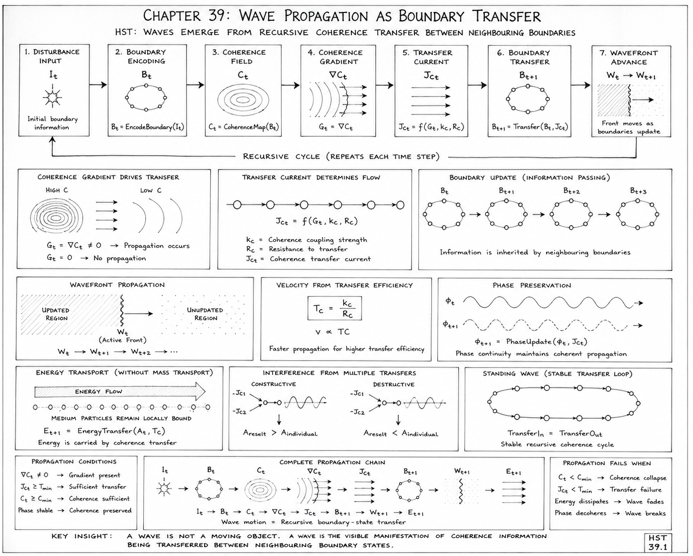
Figure 39.1 illustrates the HST interpretation of wave propagation as a recursive process of boundary-state transfer. Rather than treating waves as physical objects travelling through an independent spatial medium, the diagram models propagation as the sequential transfer of coherence information between neighbouring boundary regions.

The figure follows the complete causal chain from the initial disturbance through coherence-field generation, gradient formation, transfer-current creation, boundary updating, wavefront advancement, energy transport, interference formation, and standing-wave stabilisation.

The entire diagram is constructed around the HST principle that observable wave motion emerges from recursive coherence transfer rather than material displacement.

The diagram begins with the disturbance source:

\[ I_t \]

This represents the initial information injection into the system.

Examples include:

The disturbance introduces a local change in boundary structure.

At this stage no wave exists.

Only information has been introduced into the boundary network.

The disturbance is encoded into a local boundary state:

\[ B_t = \mathrm{EncodeBoundary}(I_t) \]

The circular boundary symbol shown in the diagram represents the first coherent structure created by the disturbance.

Within HST, all physical propagation begins from encoded boundary information rather than from moving particles.

The boundary therefore acts as the initial storage location for the incoming disturbance.

The encoded boundary generates a coherence field:

\[ C_t = \mathrm{CoherenceMap}(B_t) \]

This region is illustrated using expanding concentric contours.

These contours represent the distribution of coherence surrounding the encoded boundary.

The coherence field defines how strongly neighbouring regions are informationally aligned.

The field serves as the propagation landscape through which coherence transfer will occur.

The next section shows the formation of a coherence gradient:

\[ G_t = \nabla C_t \]

The diagram depicts regions of high coherence and low coherence connected by directional arrows.

This gradient represents the informational imbalance that drives propagation.

A key principle illustrated here is:

\[ \nabla C_t \neq 0 \]

A non-zero gradient indicates that neighbouring boundary regions possess different coherence states.

Without this imbalance, no transfer pressure exists and propagation cannot occur.

The gradient therefore acts as the fundamental driver of wave formation.

The transfer-current section introduces:

\[ J_C = f\!\left( G_t,\, k_C,\, R_C \right) \]

The arrows connecting neighbouring nodes represent directional coherence flow.

This is one of the most important elements in the entire figure.

The transfer current is not:

Instead it represents the transfer of coherence information between adjacent boundaries.

The diagram visually communicates that propagation emerges from information movement rather than object movement.

The sequence:

\[ B_t \rightarrow B_{t+1} \rightarrow B_{t+2} \rightarrow B_{t+3} \]

illustrates successive boundary inheritance.

Each boundary passes its coherence state to neighbouring regions.

The diagram shows multiple copies of the boundary structure because the information pattern is being reconstructed repeatedly across space.

This section provides the geometric basis for apparent motion.

Nothing physically travels across the entire system.

Instead neighbouring regions continuously inherit updated boundary states.

The advancing wavefront is represented by the dividing surface between updated and non-updated regions:

\[ W_t \rightarrow W_{t+1} \]

The shaded side of the diagram represents boundaries that have already received the coherence update.

The unshaded region represents boundaries that have not yet been updated.

The moving interface appears experimentally as a propagating wave.

Within HST, however, the wavefront is interpreted as the active boundary of recursive information transfer.

The front moves because the update process moves.

Not because an object moves.

The velocity block introduces:

\[ T_C = \frac{R_C}{k_C} \]

and

\[ v \propto T_C \]

This section explains how propagation speed emerges from transfer efficiency.

The diagram emphasises that velocity depends upon:

rather than upon purely geometric motion.

Fast propagation corresponds to highly efficient boundary communication.

Slow propagation corresponds to inefficient transfer pathways.

The figure therefore reinterprets wave velocity as an information-transfer rate.

The sinusoidal structures shown in the phase section represent:

\[ \phi_t \]

and

\[ \phi_{t+1} \]

The diagram illustrates that neighbouring boundary updates must preserve phase relationships.

Phase continuity allows the system to maintain coherent propagation across large distances.

Without phase preservation:

This section demonstrates how information retains structural consistency during transfer.

The energy transport section highlights a major feature of wave behaviour.

The diagram shows energy moving through the system while the medium remains locally constrained.

The governing relation is:

\[ E_{t+1} = \mathrm{EnergyTransfer} \!\left( A_t,\, T_C \right) \]

This illustrates why:

The diagram visually separates energy transport from material transport.

This distinction is central to the HST interpretation.

The interference section depicts multiple transfer currents converging on a common boundary.

Constructive interference occurs when coherence updates reinforce one another.

Destructive interference occurs when competing updates cancel.

The figure demonstrates that interference emerges naturally from boundary-update reconciliation.

The resulting pattern reflects the coherence structure of the transfer network rather than the collision of independent wave objects.

The final major process shown in the figure is standing-wave formation.

The closed-loop structure represents a stable recursive transfer cycle.

The governing condition is:

\[ \mathrm{Transfer}_{\mathrm{In}} = \mathrm{Transfer}_{\mathrm{Out}} \]

Under this condition the coherence transfer process becomes self-sustaining.

Information continuously circulates while maintaining equilibrium.

The standing wave therefore appears as a dynamically stable coherence attractor.

Within HST, standing waves are interpreted as persistent transfer loops rather than overlapping travelling oscillations.

The lower-left section summarises the requirements for successful propagation.

These include:

\[ \nabla C_t \neq 0 \]

\[ J_C \geq T_{\min} \]

\[ C_t \geq C_{\min} \]

These conditions ensure:

The diagram therefore establishes the minimum requirements for wave existence.

The lower-right section describes situations in which propagation ceases.

Examples include:

\[ C_t < C_{\min} \]

which produces coherence collapse,

and

\[ J_C < T_{\min} \]

which prevents effective transfer.

These conditions correspond physically to damping, attenuation, absorption, or decoherence.

The wave disappears because the boundary-transfer process can no longer sustain itself.

The entire diagram can be summarised by the propagation chain:

\[ I_t \rightarrow B_t \rightarrow C_t \rightarrow \nabla C_t \rightarrow J_C \rightarrow B_{t+1} \rightarrow W_{t+1} \rightarrow E_{t+1} \]

This chain represents the complete HST mechanism of wave formation.

The figure demonstrates that wave propagation emerges from recursive coherence transfer between neighbouring boundary states. Observable motion is produced by successive boundary updates, energy transport is carried by coherence transfer currents, interference emerges from competing updates, and standing waves arise from stable transfer loops.

The central conclusion illustrated by the diagram is therefore:

Within HST, wave propagation is reinterpreted as a recursive information-transfer process operating across a dynamic network of coherence boundaries, with apparent motion emerging from boundary inheritance rather than material displacement through space.

\[ I_t \rightarrow B_t \rightarrow C_t \rightarrow \nabla C_t \rightarrow J_C \rightarrow B_{t+1} \rightarrow W_{t+1} \rightarrow E_{t+1} \]

The Wave Propagation as Boundary Transfer flow is guaranteed to execute successfully if and only if a valid boundary disturbance generates a non-zero coherence gradient capable of producing sufficient coherence transfer between neighbouring boundary states while maintaining coherence, transfer efficiency, and phase stability throughout the propagation cycle.

The execution path is defined by:

\[ I_t \rightarrow B_t \rightarrow C_t \rightarrow \nabla C_t \rightarrow J_C \rightarrow B_{t+1} \rightarrow W_{t+1} \rightarrow E_{t+1} \]

where every stage must complete successfully before the next stage can execute.

Successful propagation requires all of the following conditions to remain true simultaneously:

\[ I_t \neq \emptyset \]

The system must receive an initial disturbance capable of generating a boundary-state modification.

Without information input, propagation cannot begin.

\[ B_t = \mathrm{EncodeBoundary}(I_t) \]

The disturbance must successfully map into a coherent boundary structure.

Boundary formation is the first executable state of the propagation chain.

\[ C_t = \mathrm{CoherenceMap}(B_t) \]

A valid coherence field must emerge from the encoded boundary.

Without a coherence field there can be no gradient formation.

\[ \nabla C_t \neq 0 \]

A wave can only propagate when neighbouring regions possess differing coherence states.

If:

\[ \nabla C_t = 0 \]

then:

\[ J_C = 0 \]

and propagation cannot occur.

\[ J_C \geq T_{\min} \]

The coherence transfer current must exceed the minimum transfer requirement.

This guarantees that information can successfully move between neighbouring boundaries.

Insufficient transfer results in wave attenuation and eventual termination.

\[ C_t \geq C_{\min} \]

The coherence field must remain above the minimum coherence threshold.

This condition ensures that the boundary network remains structurally connected throughout propagation.

\[ \left| \Delta \phi_t \right| \leq \phi_{\max} \]

Phase drift must remain within acceptable limits.

Phase preservation guarantees:

\[ T_C = \frac{R_C}{k_C} \]

and

\[ T_C > 0 \]

The medium must retain a positive transfer efficiency.

Neighbouring boundaries must remain capable of exchanging information.

If all execution conditions remain satisfied, the flow guarantees production of:

\[ B_{t+1} \]

Neighbouring boundaries inherit the propagated coherence structure.

\[ W_t \rightarrow W_{t+1} \]

The active propagation front advances.

\[ E_{t+1} \]

Energy is transported through the coherence network.

\[ \phi_t \rightarrow \phi_{t+1} \]

Wave continuity is preserved.

\[ B_t \rightarrow B_{t+1} \rightarrow B_{t+2} \rightarrow B_{t+3} \rightarrow \cdots \]

The system continues propagating indefinitely until a failure condition is encountered.

Execution is formally terminated if any of the following conditions occur.

\[ C_t < C_{\min} \]

Result:

\[ \mathrm{Execution} = \mathrm{FAIL} \]

The boundary network loses structural integrity.

\[ \nabla C_t = 0 \]

Result:

\[ J_C = 0 \]

No propagation force remains.

\[ J_C < T_{\min} \]

Result:

Information transfer becomes insufficient for propagation.

\[ T_C \rightarrow 0 \]

Result:

\[ v \rightarrow 0 \]

The propagation mechanism ceases.

\[ \left| \Delta \phi_t \right| > \phi_{\max} \]

Result:

WaveStructure→Collapse

The coherence structure can no longer maintain a stable wave.

The Wave Propagation as Boundary Transfer flow executes successfully if and only if:

\[ I_t \neq \emptyset \]

\[ \nabla C_t \neq 0 \]

\[ J_C \geq T_{\min} \]

\[ C_t \geq C_{\min} \]

\[ \left| \Delta \phi_t \right| \leq \phi_{\max} \]

\[ T_C > 0 \]

\[ I_t \rightarrow B_t \rightarrow C_t \rightarrow \nabla C_t \rightarrow J_C \rightarrow B_{t+1} \rightarrow W_{t+1} \]

Under these conditions the recursive update sequence

is guaranteed to remain executable, producing sustained wave propagation through recursive boundary-state transfer.

Execution(St​)⟺(It​=∅)∧(∇Ct​=0)∧(JC​≥Tmin​)∧(Ct​≥Cmin​)∧(TC​>0)∧(∣Δϕt​∣≤ϕmax​)

When these conditions hold, the flow guarantees that wave motion emerges as a continuously advancing sequence of coherence-boundary updates, transporting energy and information through recursive transfer rather than through the displacement of material substance.

This guarantee remains valid for mechanical, acoustic, electromagnetic, and quantum-wave implementations within the HST framework.