
Chapter 28
Thermodynamic Reformulation

Entropy as Coherence Dispersion
Author: Mark Higgins
© Mark Anthony Higgins 11 October 2025
Revised Date: 29 May 2026
Audio Overview

Introduction

Thermodynamics is one of the most successful frameworks in science, describing the behaviour of energy, heat, work, entropy, and equilibrium across physical systems. From steam engines and chemical reactions to biological organisms and cosmological evolution, thermodynamic laws govern how systems change over time and how energy is redistributed throughout nature.

Classical thermodynamics provides powerful predictive tools, yet many of its central concepts—particularly entropy, irreversibility, and the arrow of time—are often treated as emergent statistical phenomena rather than consequences of a deeper structural process. While statistical mechanics explains how macroscopic thermodynamic behaviour arises from microscopic states, it does not necessarily explain why systems consistently evolve toward particular classes of configurations.

Flow Algebra approaches thermodynamics from a different perspective. Rather than treating thermodynamic behaviour primarily as energy exchange between particles, it interprets thermodynamic evolution as recursive coherence redistribution occurring within constrained state spaces.

The Need for a Structural Reformulation

Traditional thermodynamics focuses on measurable quantities:

  • Energy
  • Heat
  • Work
  • Temperature
  • Entropy

These quantities successfully describe system behaviour but do not explicitly identify the recursive mechanism responsible for thermodynamic evolution.

Flow Algebra seeks to identify the structural process beneath these observations.

The central question becomes:

What determines which future states a thermodynamic system can enter?

Rather than beginning with energy transfer alone, Flow Algebra begins with recursive state continuation.

Every physical system occupies a current state and must transition into a future state while preserving fundamental constraints. Thermodynamic behaviour emerges from the selection and propagation of these admissible continuations.

Thermodynamic Systems as Recursive Structures

Within Flow Algebra, a thermodynamic system is represented as:

\[ S_t = (I_t, R, B, K) \]

where:

  • ItI_t represents the current information state.
  • RR represents the governing transformation rules.
  • BB represents boundary constraints.
  • KK represents preserved invariants.

The future evolution of the system is determined not by arbitrary motion but by the set of admissible continuations generated from these recursive components.

Thermodynamics therefore becomes a special case of recursive state evolution.

Energy as Continuation Capacity

In conventional physics, energy is often interpreted as the capacity to perform work.  Within Flow Algebra, energy may be viewed more fundamentally as:

The capacity of a system to generate admissible future continuations.

A highly energetic system possesses many possible pathways for future evolution.  A low-energy system possesses fewer admissible continuations and therefore less freedom for future state construction.

Energy thus becomes directly connected to the geometry of recursive state space.

Entropy as Coherence Dispersion

One of the most significant shifts introduced by the thermodynamic reformulation concerns entropy.  Traditional thermodynamics frequently describes entropy as disorder.

Flow Algebra instead defines entropy as:

The dispersion of coherence across admissible continuation space.

As systems evolve:

  • Coherence becomes distributed across larger regions of state space.
  • Local structure may dissolve.
  • Future continuations become increasingly numerous.
  • State density spreads across admissible configurations.

Entropy growth therefore reflects increasing coherence dispersion rather than increasing disorder alone.  This interpretation preserves classical thermodynamic predictions while providing a structural explanation for entropy production.

Entropy growth therefore reflects increasing coherence dispersion rather than increasing disorder alone.

This interpretation preserves classical thermodynamic predictions while providing a structural explanation for entropy production.

Equilibrium as Stable Continuation Density

Classical equilibrium occurs when macroscopic variables cease changing over time.

Within Flow Algebra, equilibrium corresponds to a condition where recursive continuation density becomes stable.

In this state:

  • Admissible future states remain available.
  • Constraint satisfaction is maintained.
  • Large-scale coherence gradients vanish.
  • Recursive evolution no longer generates significant macroscopic reorganisation.

Equilibrium is therefore not the absence of activity.

Instead, it is the emergence of a dynamically stable continuation structure.

Telephone:
01377 236594

Irreversibility as Continuation Asymmetry

One of the longstanding puzzles of thermodynamics concerns irreversibility. Microscopic physical laws are often reversible, yet macroscopic thermodynamic processes exhibit a preferred direction.

Flow Algebra explains this through continuation asymmetry.

As recursive systems evolve:

  • Certain continuation pathways remain admissible.
  • Reverse pathways rapidly become inaccessible.
  • Coherence disperses into increasingly distributed configurations.
  • Reconstruction of previous states becomes progressively less probable.

Irreversibility therefore emerges naturally from the geometry of admissible continuation space.  The arrow of thermodynamic evolution reflects asymmetry in recursive continuation availability.

Heat Flow as Coherence Redistribution

Heat transfer can also be reformulated within the Flow Algebra framework. Conventionally, heat flows from higher temperature regions to lower temperature regions.

Structurally, this process represents:

The redistribution of coherence gradients across a constrained boundary system.

Regions of concentrated coherence transfer admissible continuation capacity into neighbouring regions until gradient imbalance is reduced.

Heat flow therefore becomes a manifestation of recursive coherence equalisation.

A Unified Description of Thermodynamic Behaviour

This reformulation allows diverse thermodynamic phenomena to be understood through a common recursive mechanism.

Examples include:

  • Heat transfer
  • Diffusion
  • Chemical reactions
  • Phase transitions
  • Biological metabolism
  • Atmospheric dynamics
  • Cosmological entropy production

Each process represents a different manifestation of recursive coherence redistribution operating under distinct boundary conditions.

The governing mechanism remains identical.

Relationship to Classical Thermodynamics

The purpose of this reformulation is not to replace classical thermodynamics.  Classical thermodynamics remains fully valid as an observational and predictive framework.

Instead, Flow Algebra provides a deeper structural interpretation that explains why thermodynamic laws emerge.

Under this view:

  • Energy describes continuation capacity.
  • Entropy describes coherence dispersion.
  • Equilibrium describes stable continuation density.
  • Irreversibility describes continuation asymmetry.
  • Thermodynamic evolution describes recursive coherence redistribution.

The classical laws become observable consequences of deeper recursive dynamics.

Chapter Overview

This chapter develops a complete thermodynamic reformulation within Flow Algebra.

The following sections will demonstrate how entropy growth, equilibrium formation, heat transfer, energy flow, and irreversible processes emerge directly from recursive state evolution.

By reframing thermodynamics as a theory of coherence redistribution within admissible continuation space, the chapter establishes a unified structural foundation capable of describing both classical thermodynamic behaviour and more general recursive systems.

Thermodynamics therefore becomes more than a theory of heat and energy.

It becomes a theory of how coherence evolves through constrained recursive reality.

flow "ThermodynamicReformulation" v1.0

# ------------------------------------------------------------
# PURPOSE
# ------------------------------------------------------------
# Reformulates thermodynamic evolution as recursive coherence
# redistribution through admissible continuation space.
#
# Classical thermodynamic quantities are interpreted structurally:
# energy        → continuation capacity
# entropy       → coherence dispersion
# heat flow     → coherence-gradient redistribution
# equilibrium   → stable continuation density
# irreversibility → continuation asymmetry

# ------------------------------------------------------------
# STATE
# ------------------------------------------------------------
state S_t:
  I_t: current_information_state
  R: transformation_rules
  B: thermodynamic_boundary_constraints
  K: conserved_invariants

# ------------------------------------------------------------
# PARAMETERS
# ------------------------------------------------------------
params:
  C_min: minimum_coherence_threshold
  Sigma_max: maximum_recoverable_entropy
  epsilon: stability_tolerance
  beta: inverse_temperature_parameter

# ------------------------------------------------------------
# CORE DEFINITIONS
# ------------------------------------------------------------
define E_t:
  E_t = expand(I_t, R)

define V_t:
  V_t = { x in E_t | x satisfies (B and K) }

define Omega_t:
  Omega_t = coherence_density(I_t, B, K)

define Sigma_t:
  Sigma_t = dispersion(Omega_t over V_t)

define Energy_t:
  Energy_t = continuation_capacity(V_t)

define HeatFlow_t:
  HeatFlow_t = redistribute(coherence_gradient(I_t), B)

# ------------------------------------------------------------
# THERMODYNAMIC SELECTION
# ------------------------------------------------------------
select x_star from V_t:
  x_star = argmax_x P(x | I_t, R, B, K, beta)

update:
  I_{t+1} = update(I_t, x_star)
  S_{t+1} = (I_{t+1}, R, B, K)

# ------------------------------------------------------------
# INVARIANTS
# ------------------------------------------------------------
invariants:
  V_t != empty
  Omega_t >= C_min
  x_star satisfies (B and K)
  conserved(K) == true
  Delta Sigma_total >= 0

# ------------------------------------------------------------
# PROCESS
# ------------------------------------------------------------
process ThermodynamicEvolution:

  step 1:
    generate E_t from I_t using R

  step 2:
    filter E_t through B and K to produce V_t

  step 3:
    measure Omega_t as recoverable coherence density

  step 4:
    compute Sigma_t as coherence dispersion

  step 5:
    compute Energy_t as available continuation capacity

  step 6:
    redistribute coherence gradients as HeatFlow_t

  step 7:
    if V_t != empty and Omega_t >= C_min:
      select x_star from V_t
      update I_t to I_{t+1}
      continue

  step 8:
    if V_t == empty:
      Execution(S_t) = FAIL

  step 9:
    if Omega_t < C_min:
      Execution(S_t) = THERMODYNAMIC_COLLAPSE

  step 10:
    if abs(Delta Sigma_t) <= epsilon:
      state = EQUILIBRIUM

# ------------------------------------------------------------
# EQUILIBRIUM CONDITION
# ------------------------------------------------------------
equilibrium:
  abs(Delta Sigma_t) <= epsilon
  coherence_gradient(I_t) ≈ 0
  continuation_density(V_t) stable
  Execution(S_t) = STABLE

# ------------------------------------------------------------
# IRREVERSIBILITY CONDITION
# ------------------------------------------------------------
irreversibility:
  forward_continuations = count(V_t)
  reverse_continuations = count(reverse_admissible(I_{t+1}, I_t))

  if forward_continuations >> reverse_continuations:
    arrow_of_time = forward
    reverse_reconstruction = improbable

# ------------------------------------------------------------
# FAILURE CONDITIONS
# ------------------------------------------------------------
failures:

  no_admissible_continuation:
    condition: V_t == empty
    result: Execution(S_t) = FAIL

  coherence_collapse:
    condition: Omega_t < C_min
    result: Execution(S_t) = THERMODYNAMIC_COLLAPSE

  unrecoverable_entropy:
    condition: Sigma_t > Sigma_max
    result: local_structure = unrecoverable

# ------------------------------------------------------------
# EXECUTION GUARANTEE
# ------------------------------------------------------------
guarantee:
  Execution(S_t) iff V_t != empty and Omega_t >= C_min

  If admissible continuations exist and coherence remains above
  threshold, thermodynamic evolution continues.

  If no admissible continuation exists, execution fails.

  If coherence falls below threshold, the system collapses into
  thermodynamic disorder or unrecoverable dispersion.

What This Flow Implements

Overview

The Thermodynamic Reformulation Flow provides a structural description of thermodynamic behaviour using the recursive state-transition framework of Flow Algebra. Rather than treating thermodynamics solely as the study of heat, energy, and entropy, the flow models thermodynamic evolution as the progression of admissible continuations through a constrained recursive state space.

The implementation establishes a direct correspondence between classical thermodynamic phenomena and recursive coherence dynamics, allowing energy transfer, entropy growth, equilibrium formation, and irreversible processes to be described within a unified structural framework.

The flow therefore serves as a formal mechanism for expressing thermodynamic systems as recursive coherence-distribution processes.

Recursive Thermodynamic State Construction

The flow begins by defining a thermodynamic system as:

\[ S_t = (I_t, R, B, K) \]

where:

  • ItI_t represents the current information state.
  • RR represents transformation rules.
  • BB represents thermodynamic boundary constraints.
  • KK represents conserved invariants.

This construction provides the complete recursive description of the thermodynamic system at time tt.  Every subsequent thermodynamic process is derived from this state definition.

Admissible Continuation Generation

The flow generates possible future thermodynamic configurations through:

\[ E_t = \operatorname{expand}(I_t, R) \]

This operation creates all candidate continuations permitted by the governing thermodynamic rules.

Examples include:

  • Heat redistribution pathways
  • Diffusion pathways
  • Chemical reaction possibilities
  • Phase-transition candidates
  • Equilibrium trajectories

The expansion stage defines the future thermodynamic possibility space before constraints are applied.

Thermodynamic Boundary Filtering

Not all generated continuations are physically permissible.  The flow therefore constructs the admissible continuation set:

\[ V_t = \{x \in E_t \mid x \models (B \land K)\} \]

This filtering stage ensures that every admissible thermodynamic continuation:

  • Obeys physical boundaries.
  • Preserves conserved quantities.
  • Satisfies thermodynamic constraints.
  • Maintains invariant system requirements.

The flow therefore guarantees structural consistency throughout thermodynamic evolution.

Coherence Density Measurement

The flow introduces a structural measure:

\[ \Omega_t = \operatorname{coherence\_density}(I_t, B, K) \]

This quantity measures the recoverable coherence present within the current thermodynamic state.  Coherence density acts as the primary indicator of thermodynamic organisation.

High values correspond to:

  • Strong structural organisation
  • Stable thermodynamic order
  • Recoverable information content

Low values correspond to:

  • Increasing dispersion
  • Reduced recoverability
  • Thermodynamic degradation

The flow continuously monitors coherence density during execution.

Entropy as Coherence Dispersion

A central feature of the implementation is the reformulation of entropy.

The flow defines entropy structurally as:

\[ \Sigma_t = \operatorname{dispersion}(\Omega_t \ \text{over} \ V_t) \]

Rather than interpreting entropy as disorder alone, the implementation treats entropy as the distribution of coherence throughout admissible continuation space.

Under this formulation:

  • Entropy growth corresponds to coherence dispersion.
  • Entropy reduction corresponds to coherence concentration.
  • Equilibrium corresponds to stable dispersion density.

This provides a structural interpretation of the Second Law of Thermodynamics.

Energy as Continuation Capacity

The flow reinterprets energy as:

\[ \mathrm{Energy}_t = \operatorname{continuation\_capacity}(V_t) \]

This definition measures the number and accessibility of future admissible continuations available to the system.

Within the implementation:

  • High energy states possess greater continuation flexibility.
  • Low energy states possess fewer admissible continuations.
  • Energy transfer modifies future continuation capacity.

This creates a direct relationship between thermodynamics and recursive state-space geometry.

Heat Flow as Coherence Redistribution

The implementation models heat transfer through:

\[ \mathrm{Energy}_t = \operatorname{continuation\_capacity}(V_t) \]

Heat is therefore represented as the redistribution of coherence gradients across system boundaries.  This interpretation captures classical heat-flow behaviour while embedding it within the recursive coherence framework.

Heat transfer becomes a structural process rather than merely an energetic one.

Equilibrium Formation

The flow formally implements thermodynamic equilibrium through the condition:

\[ \left|\Delta \Sigma_t\right| \leq \epsilon \]

combined with:

\[ \operatorname{coherence\_gradient}(I_t) \approx 0 \]

Equilibrium is therefore identified as a state in which:

  • Coherence gradients vanish.
  • Entropy growth stabilises.
  • Continuation density becomes stationary.
  • Large-scale thermodynamic reorganisation ceases.

The implementation treats equilibrium as a dynamically stable recursive state rather than a static endpoint.

Irreversibility and the Arrow of Time

The flow implements thermodynamic irreversibility through continuation asymmetry.

It evaluates:

  • Forward admissible continuations.
  • Reverse admissible continuations.

When:

\[ \mathrm{Forward} \gg \mathrm{Reverse} \]

the system exhibits a preferred thermodynamic direction.

The implementation therefore explains the arrow of time as an emergent property of recursive continuation geometry rather than a fundamental physical law.

Irreversibility arises because reverse continuations become progressively less admissible as coherence disperses.

Thermodynamic Failure Detection

The flow includes explicit thermodynamic failure conditions.

These include:

No Admissible Continuation

\[ V_t = \emptyset \]

resulting in:

\[ \operatorname{Execution}(S_t) = \mathrm{FAIL} \]

Coherence Collapse

\[ \Omega_t < C_{\min} \]

resulting in:

\[ \operatorname{Execution}(S_t) = \mathrm{THERMODYNAMIC\_COLLAPSE} \]

Unrecoverable Entropy

\[ \Sigma_t > \Sigma_{\max} \]

resulting in irreversible loss of recoverable structure.

These mechanisms allow the framework to distinguish between stable thermodynamic evolution and structural breakdown.

Unified Thermodynamic Execution

The complete implementation unifies:

  • Energy transfer
  • Heat flow
  • Entropy growth
  • Equilibrium formation
  • Irreversibility
  • Thermodynamic stability
  • Structural collapse

under a single recursive coherence model.

Classical thermodynamic behaviour emerges naturally from admissible continuation selection operating within constrained recursive state spaces.

Scientific Significance

The significance of this flow lies in its reformulation of thermodynamics as a coherence-distribution process rather than solely an energy-distribution process.

Within Flow Algebra:

  • Energy becomes continuation capacity.
  • Entropy becomes coherence dispersion.
  • Heat becomes coherence redistribution.
  • Equilibrium becomes stable continuation density.
  • Irreversibility becomes continuation asymmetry.

The flow therefore provides a unified structural foundation for thermodynamic behaviour, connecting classical thermodynamics to the broader recursive principles that govern physical, computational, and informational systems.

How to Read This Flow

Purpose of the Flow

The Thermodynamic Reformulation Flow describes thermodynamic evolution as a recursive coherence-distribution process. Rather than viewing thermodynamics solely through heat, energy, and particle interactions, the flow represents thermodynamic behaviour as the propagation of admissible state transitions through a constrained recursive system.

The flow should be read from top to bottom as a complete execution pathway that begins with a thermodynamic state, generates possible future continuations, evaluates their admissibility, measures coherence and entropy, and then selects a valid continuation for the next thermodynamic update.

Each section represents a specific structural component of thermodynamic evolution.

Step 1 — Define the Thermodynamic State

The flow begins with the system definition:

\[ S_t = (I_t, R, B, K) \]

where:

  • ItI_t is the current thermodynamic information state.
  • RR is the set of thermodynamic transformation rules.
  • BB is the set of boundary constraints.
  • KK is the set of conserved invariants.

This equation represents the complete thermodynamic description of the system at time tt.

When reading the flow, all subsequent operations are derived from this state definition.

Step 2 — Generate Future Thermodynamic Possibilities

The next operation is:

\[ E_t = \operatorname{expand}(I_t, R) \]

This stage generates all possible future thermodynamic continuations permitted by the governing rules.

Conceptually, this represents the system asking:

"What thermodynamic states could occur next?"

Examples include:

  • Heat redistribution pathways.
  • Diffusion possibilities.
  • Chemical reaction outcomes.
  • Phase transition candidates.
  • Relaxation trajectories.

At this stage no filtering has yet occurred.  The system simply constructs the future possibility space.

Step 3 — Apply Thermodynamic Constraints

The generated possibilities are filtered through:

\[ V_t = \{x \in E_t \mid x \models (B \land K)\} \]

This is the admissibility stage.

Only continuations that satisfy:

  • Boundary constraints (BB)
  • Conserved invariants (KK)

are retained.
When reading the flow, VtV_t should be interpreted as:

The set of physically valid future thermodynamic states.

Any continuation violating thermodynamic requirements is removed.

Step 4 — Measure Coherence Density

The flow then computes:

\[ \Omega_t = \operatorname{coherence\_density}(I_t, B, K) \]

This quantity measures the amount of recoverable structural organisation present within the thermodynamic system.

Interpretation:

  • High Ωt\Omega_t → highly organised system.
  • Moderate Ωt\Omega_t → partially dispersed system.
  • Low Ω t ​ → degraded thermodynamic structure.

When reading the flow, coherence density functions as the primary indicator of thermodynamic stability.

Step 5 — Compute Entropy

The next operation calculates entropy:

\[ \Sigma_t = \operatorname{dispersion}(\Omega_t \ \text{over} \ V_t) \]

Within the thermodynamic reformulation:
Entropy is interpreted as coherence dispersion.

This step measures how widely coherence is distributed throughout admissible continuation space.

Interpretation:

  • Small dispersion → concentrated coherence.
  • Large dispersion → distributed coherence.
  • Increasing dispersion → entropy growth.

When reading the flow, this stage provides the structural equivalent of entropy measurement.

Step 6 — Compute Continuation Capacity

The flow then evaluates:

\[ \mathrm{Energy}_t = \operatorname{continuation\_capacity}(V_t) \]

This quantity represents the number and accessibility of future admissible continuations available to the system.

Within the reformulation:
Energy corresponds to continuation capacity.

Interpretation:

  • Large continuation capacity → high available energy.
  • Small continuation capacity → low available energy.

This stage links thermodynamic energy to recursive state-space structure.

Step 7 — Evaluate Heat Redistribution

The flow next calculates:

\[ \mathrm{HeatFlow}_t = \operatorname{redistribute} \!\left( \operatorname{coherence\_gradient}(I_t), B \right) \]

This operation models heat transfer.

Rather than treating heat solely as energy movement, the flow interprets heat as the redistribution of coherence gradients across system boundaries.

When reading this stage:

  • Large gradients produce strong heat flow.
  • Small gradients produce weak heat flow.
  • Vanishing gradients indicate approach toward equilibrium.

Step 8 — Select the Next Thermodynamic Continuation

After all measurements have been completed, the flow selects:

\[ x^{*} = \underset{x \in V_t}{\operatorname{arg\,max}} \; P\!\left( x \mid I_t, R, B, K, \beta \right) \]

This is the continuation-selection stage.

The system chooses the most probable admissible continuation according to its recursive conditions.

Importantly:

  • Selection occurs only after admissibility filtering.
  • Invalid states cannot be selected.
  • Conserved invariants remain preserved.

This guarantees structurally valid thermodynamic evolution.

Step 9 — Update the Thermodynamic State

The selected continuation updates the system:

\[ I_{t+1} = \operatorname{update}(I_t, x^{*}) \]

and therefore:

\[ S_{t+1} = \left( I_{t+1}, R, B, K \right) \]

This produces the next thermodynamic state.
The flow then repeats recursively.

When reading the flow, this marks the completion of one thermodynamic evolution cycle.

Step 10 — Evaluate Equilibrium

The equilibrium section checks whether:

\[ \left|\Delta \Sigma_t\right| \leq \epsilon \]

and

\[ \operatorname{coherence\_gradient}(I_t) \approx 0 \]

If both conditions are satisfied:

\[ \operatorname{Execution}(S_t) = \mathrm{STABLE} \]

This indicates thermodynamic equilibrium.

The system remains dynamically active but no longer undergoes significant large-scale reorganisation.

Step 11 — Evaluate Irreversibility

The flow then compares:

Forward Continuations

with

Reverse Continuations

If:

Forward≫Reverse

the system exhibits thermodynamic irreversibility.

When reading this section, the arrow of time emerges from continuation asymmetry rather than being imposed externally.

The system naturally evolves toward regions of state space where reverse reconstruction becomes increasingly unlikely.

Step 12 — Check Failure Conditions

The final stage evaluates thermodynamic viability.

No Admissible Continuation

\[ V_t = \emptyset \]

produces:

\[ \operatorname{Execution}(S_t) = \mathrm{FAIL} \]

Coherence Collapse

\[ \Omega_t < C_{\min} \]

produces:

\[ \operatorname{Execution}(S_t) = \mathrm{THERMODYNAMIC\_COLLAPSE} \]

Unrecoverable Entropy

\[ \Sigma_t > \Sigma_{\max} \]

produces irreversible structural degradation.

These conditions determine whether thermodynamic evolution can continue.

Reading the Flow as a Complete Thermodynamic Cycle

The entire flow can therefore be read as:

St​→Et​→Vt​→Ωt​→Σt​→Energyt​→HeatFlowt​→x∗→St+1​

This sequence represents one complete cycle of recursive thermodynamic evolution.

The system:
  • 1. Defines its current state.
  • 2. Generates future possibilities.
  • 3. Filters admissible continuations.
  • 4. Measures coherence.
  • 5. Computes entropy.
  • 6. Computes continuation capacity.
  • 7. Redistributes coherence gradients.
  • 8. Selects a valid continuation.
  • 9. Updates the state.
  • 10. Repeats recursively.

Scientific Interpretation

From a scientific perspective, this flow implements a structural reformulation of thermodynamics in which:

  • Energy becomes continuation capacity.
  • Entropy becomes coherence dispersion.
  • Heat becomes coherence redistribution.
  • Equilibrium becomes stable continuation density.
  • Irreversibility becomes continuation asymmetry.

The flow should therefore be read not as a simulation of particles or heat alone, but as a recursive execution engine governing the evolution of thermodynamic coherence through admissible continuation space.

Flow → Equation Tri-Mapping

Flow Stage Flow Algebra Operation Equation Mapping
Thermodynamic State Definition Recursive thermodynamic system construction \( S_t=(I_t,R,B,K) \)
Future State Expansion Candidate thermodynamic continuation generation \( E_t=\operatorname{expand}(I_t,R) \)
Admissibility Filtering Boundary and invariant constrained selection \( V_t=\{x\in E_t\mid x\models(B\land K)\} \)
Coherence Density Measurement Recoverable thermodynamic organisation \( \Omega_t=\operatorname{coherence\_density}(I_t,B,K) \)
Entropy Definition Coherence dispersion metric \( \Sigma_t=\operatorname{dispersion}(\Omega_t\ \text{over}\ V_t) \)
Energy Definition Continuation capacity measurement \( Energy_t=\operatorname{continuation\_capacity}(V_t) \)
Heat Flow Definition Coherence-gradient redistribution \( HeatFlow_t=\operatorname{redistribute}(\operatorname{coherence\_gradient}(I_t),B) \)
Continuation Selection Most probable admissible thermodynamic transition \( x^*=\arg\max_{x\in V_t}P(x\mid I_t,R,B,K,\beta) \)
State Update Recursive thermodynamic evolution \( I_{t+1}=\operatorname{update}(I_t,x^*) \)
Next System State Recursive continuation construction \( S_{t+1}=(I_{t+1},R,B,K) \)
Entropy Growth Law Thermodynamic coherence dispersion increase \( \Delta\Sigma_{total}\geq0 \)
Equilibrium Condition Stable entropy configuration \( |\Delta\Sigma_t|\leq\epsilon \)
Thermal Equilibrium Vanishing coherence gradients \( \operatorname{coherence\_gradient}(I_t)\approx0 \)
Stable Thermodynamic Execution Dynamically stable continuation density \( \operatorname{Execution}(S_t)=\mathrm{STABLE} \)
Irreversibility Criterion Continuation asymmetry \( N_{forward}\gg N_{reverse} \)
Arrow of Time Emergence Preferred continuation direction \( Forward\rightarrow Future \)
Continuation Capacity Reduction Energy dissipation effect \( Energy_{t+1}\leq Energy_t \)
Heat Redistribution Process Coherence equalisation across boundaries \( \nabla\Omega_t\rightarrow0 \)
Admissible Evolution Condition Valid thermodynamic continuation exists \( V_t\neq\emptyset \)
Coherence Preservation Condition Structural viability maintained \( \Omega_t\geq C_{min} \)
Execution Guarantee Condition Thermodynamic evolution remains possible \( V_t\neq\emptyset\land\Omega_t\geq C_{min} \)
Failure Condition No admissible continuation exists \( V_t=\emptyset \)
Execution Failure Recursive evolution terminates \( \operatorname{Execution}(S_t)=\mathrm{FAIL} \)
Coherence Collapse Condition Thermodynamic organisation below threshold \( \Omega_t<C_{min} \)
Thermodynamic Collapse Structural coherence failure \( \operatorname{Execution}(S_t)=\mathrm{THERMODYNAMIC\_COLLAPSE} \)
Unrecoverable Entropy Condition Excessive coherence dispersion \( \Sigma_t>\Sigma_{max} \)
Structural Degradation Loss of recoverable organisation \( Structure_{recoverable}\rightarrow0 \)
Complete Thermodynamic Cycle Full recursive thermodynamic evolution \( S_t\rightarrow E_t\rightarrow V_t\rightarrow\Omega_t\rightarrow\Sigma_t\rightarrow Energy_t\rightarrow HeatFlow_t\rightarrow x^*\rightarrow S_{t+1} \)
Thermodynamic Reformulation Principle Entropy as coherence dispersion \( Entropy\equiv Dispersion(\Omega) \)
Energy Reformulation Principle Energy as continuation capacity \( Energy\equiv ContinuationCapacity(V) \)
Heat Reformulation Principle Heat as coherence redistribution \( Heat\equiv Redistribution(\nabla\Omega) \)
Equilibrium Reformulation Principle Stable continuation density \( Equilibrium\equiv Stable(V_t) \)
Irreversibility Reformulation Principle Continuation asymmetry geometry \( Irreversibility\equiv N_{forward}\gg N_{reverse} \)

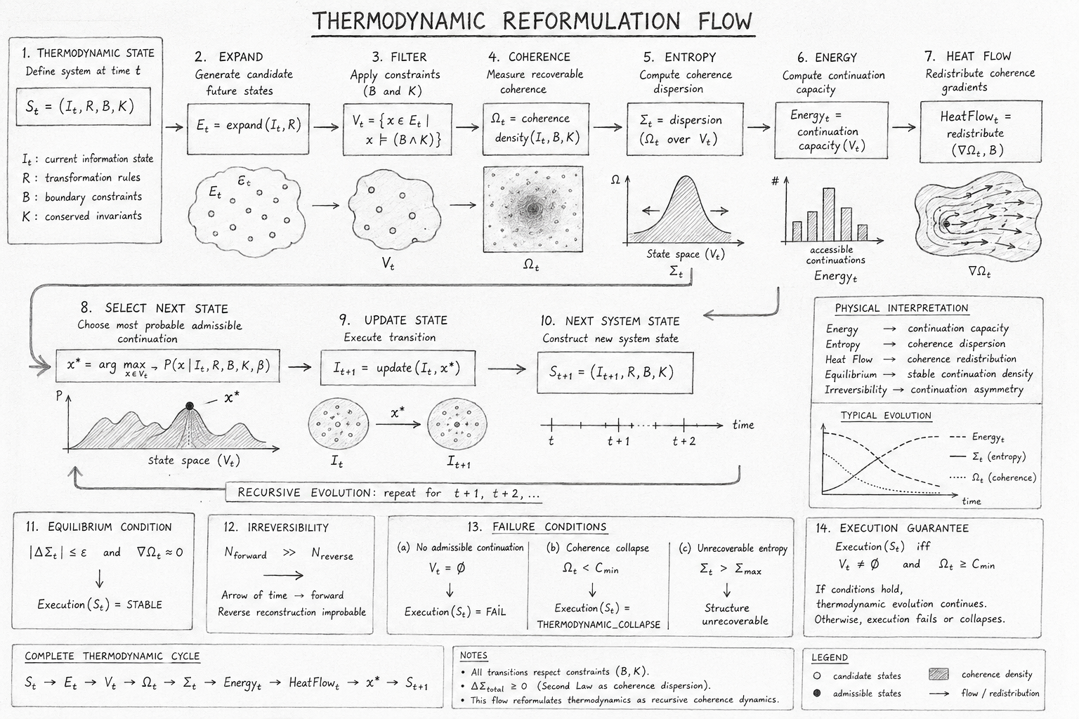
Thermodynamic Reformulation FLow

Overview

This diagram illustrates the Flow Algebra reformulation of thermodynamics as a recursive coherence-distribution process. Rather than describing thermodynamic systems solely through energy transfer and particle statistics, the figure presents thermodynamic evolution as the propagation of admissible continuations through a constrained recursive state space.

The complete thermodynamic cycle proceeds through state construction, continuation generation, admissibility filtering, coherence measurement, entropy computation, energy evaluation, heat redistribution, continuation selection, and recursive state updating. Classical thermodynamic behaviour emerges naturally from the geometry of admissible continuation space.

Thermodynamic State Construction

The process begins with the thermodynamic system definition:

\[ S_t = (I_t, R, B, K) \]

This state contains:

  • Current information state ItI_t
  • Transformation rules RR
  • Boundary constraints BB
  • Conserved invariants KK

Together these define the complete thermodynamic configuration at time tt.

The leftmost section of the diagram establishes the recursive foundation from which all subsequent thermodynamic behaviour emerges.

Expansion of Future Thermodynamic Possibilities

The next stage generates possible future continuations:

\[ E_t = \operatorname{expand}(I_t, R) \]

This operation constructs the future possibility space of the thermodynamic system.

Examples include:

  • Heat transfer pathways
  • Diffusion possibilities
  • Chemical reaction trajectories
  • Phase transition outcomes
  • Relaxation processes

The diagram represents this as a cloud of candidate states generated from the current system configuration.

Admissibility Filtering

Not every generated continuation is physically valid.  The filtering stage applies thermodynamic constraints:

\[ V_t = \{x \in E_t \mid x \models (B \land K)\} \]

Only states satisfying both:

  • Boundary constraints
  • Conserved invariants

remain admissible.

The diagram illustrates this as a reduction from many candidate states to a smaller set of valid thermodynamic continuations.

This stage guarantees physical consistency throughout execution.

Coherence Density Measurement

Once admissible continuations have been identified, the flow evaluates coherence density:

\[ \Omega_t = \operatorname{coherence\_density}(I_t, B, K) \]

This quantity measures the amount of recoverable thermodynamic organisation present within the system.

The shaded coherence field shown in the diagram represents regions of concentrated structural organisation.

High coherence density corresponds to:

  • Stable organisation
  • Recoverable information
  • Thermodynamic structure

Low coherence density corresponds to:

  • Dispersion
  • Degradation
  • Loss of recoverability

Entropy as Coherence Dispersion

The entropy stage computes:

\[ \Sigma_t = \operatorname{dispersion}(\Omega_t \ \text{over} \ V_t) \]

The diagram visualises entropy as the spreading of coherence throughout admissible continuation space.

Within the reformulation:
Entropy is not simply disorder.

Entropy is the dispersion of coherence across admissible thermodynamic configurations.

As coherence spreads, entropy increases.  As coherence concentrates, entropy decreases.

This interpretation provides a structural explanation for entropy growth and the Second Law of Thermodynamics.

Energy as Continuation Capacity

The energy stage evaluates:

\[ \mathrm{Energy}_t = \operatorname{continuation\_capacity}(V_t) \]

The histogram shown in the diagram represents the number of accessible future continuations available to the system.

Within this framework:

  • High energy corresponds to many admissible continuations.
  • Low energy corresponds to fewer admissible continuations.

Energy therefore becomes a measure of future state accessibility rather than merely stored physical quantity.

Heat Flow as Coherence Redistribution

The heat-flow section computes:

\[ \mathrm{HeatFlow}_t = \operatorname{redistribute} \!\left( \operatorname{coherence\_gradient}(I_t), B \right) \]

The curved arrows in the figure illustrate coherence moving from regions of high concentration toward regions of lower concentration.

Heat transfer is therefore interpreted as:
The redistribution of coherence gradients across thermodynamic boundaries.

The diagram visualises this process as coherence equalisation throughout the system.

Continuation Selection

After all thermodynamic quantities have been evaluated, the system selects:

\[ x^{*} = \underset{x \in V_t}{\operatorname{arg\,max}} \; P\!\left( x \mid I_t, R, B, K, \beta \right) \]

The probability distribution shown in the diagram represents the admissible continuation landscape.

The selected continuation x∗x^* corresponds to the highest-probability admissible future state.

Importantly:

  • Selection occurs only within VtV_t.
  • Invalid continuations are excluded.
  • Physical constraints remain preserved.

This guarantees thermodynamic consistency.

Recursive State Update

The selected continuation updates the system through:

\[ I_{t+1} = \operatorname{update}(I_t, x^{*}) \]

which produces:

\[ S_{t+1} = \left( I_{t+1}, R, B, K \right) \]

The timeline illustrated in the diagram represents recursive thermodynamic evolution through successive state updates.

The system continuously regenerates its future possibilities while maintaining structural consistency.

Equilibrium Formation

The equilibrium block identifies stable thermodynamic behaviour through:

\[ \left|\Delta \Sigma_t\right| \leq \epsilon \]

and

\[ \nabla \Omega_t \approx 0 \]

At equilibrium:

  • Entropy growth stabilises.
  • Coherence gradients vanish.
  • Continuation density becomes stationary.

The diagram represents this condition as a stable execution state.

Equilibrium is therefore interpreted as stable recursive continuation density rather than complete inactivity.

Irreversibility and the Arrow of Time

The irreversibility section compares:

\[ N_{\mathrm{forward}} \]

and

\[ N_{\mathrm{reverse}} \]

When:

\[ N_{\mathrm{forward}} \gg N_{\mathrm{reverse}} \]

the system develops a preferred thermodynamic direction.  The diagram shows this asymmetry as the emergence of the arrow of time.

Within the reformulation, irreversibility arises because reverse reconstructions become progressively less admissible as coherence disperses.

Failure Conditions

The lower section of the diagram identifies three thermodynamic failure modes.

No Admissible Continuation

\[ V_t = \emptyset \]

Result:

\[ \operatorname{Execution}(S_t) = \mathrm{FAIL} \]

No physically valid future state exists.

Coherence Collapse

\[ \Omega_t < C_{\min} \]

Result:

\[ \operatorname{Execution}(S_t) = \mathrm{THERMODYNAMIC\_COLLAPSE} \]

The system loses sufficient structural organisation to continue stable evolution.

Unrecoverable Entropy

\[ \Sigma_t > \Sigma_{\max} \]

Result:

Structural recovery becomes impossible.

The system enters a permanently degraded thermodynamic configuration.

Execution Guarantee

The diagram concludes with the thermodynamic execution condition:

\[ \operatorname{Execution}(S_t) \Leftrightarrow V_t \neq \emptyset \;\land\; \Omega_t \geq C_{\min} \]

This statement defines the fundamental requirement for thermodynamic continuation.

As long as:

  • Admissible continuations exist, and
  • Coherence remains above threshold,

the thermodynamic system continues evolving.


Telephone:
01377 236594

Scientific Interpretation

The diagram demonstrates that thermodynamic behaviour can be reformulated as recursive coherence dynamics operating within constrained continuation space.

Under this interpretation:

\[ \mathrm{Entropy} \equiv \mathrm{Dispersion}(\Omega) \]

\[ \mathrm{Energy} \equiv \mathrm{ContinuationCapacity}(V) \]

\[ \mathrm{Heat} \equiv \mathrm{Redistribution}(\nabla \Omega) \]

\[ \mathrm{Equilibrium} \equiv \mathrm{Stable}(V_t) \]

\[ \mathrm{Irreversibility} \equiv N_{\mathrm{forward}} \gg N_{\mathrm{reverse}} \]

The figure therefore presents a unified structural model in which entropy growth, heat transfer, equilibrium formation, and irreversible evolution emerge naturally from recursive continuation geometry rather than existing as independent thermodynamic principles.

Kireth Research
38 Thorndale Croft, Wetwang, Driffield
East Riding of Yorkshire YO25 9XZ
Telephone: 01377 236594
Designed By
