Photons and Coherence Geometry

Author: Mark Higgins
© Mark Anthony Higgins 11 October 2025

Revised Date: 15th June 2026

Audio Overview

Introduction

Photons occupy a unique position within modern physics. They are treated simultaneously as particles, waves, quantum excitations, information carriers, and the mediators of electromagnetic interaction. Despite their central role, many fundamental questions remain conceptually difficult. Why does light always travel at a fixed velocity? Why does it exhibit both wave-like and particle-like behaviour? How can a photon appear to take multiple paths while arriving as a single event?

Within conventional frameworks, these behaviours are described mathematically with extraordinary accuracy, yet the underlying physical interpretation remains fragmented between quantum mechanics, electromagnetism, and relativity.

Holographic Space-Time (HST) approaches the problem from a different foundation.

Rather than treating photons as particles moving through a pre-existing space, HST interprets photons as propagating coherence structures within an encoded boundary geometry. Light is not a small object travelling through a container called space. Instead, it is a self-maintaining coherence transfer process moving across a structured information surface.

In this framework, photons become geometric events rather than travelling objects.

From Objects to Coherence Transfer

Classical intuition imagines a photon as a tiny projectile moving from one location to another.

HST replaces this picture entirely.

A photon is interpreted as a propagating coherence disturbance that transfers information between neighbouring regions of a boundary structure.

The important entity is not the photon itself but the coherence pattern it carries.

The observable effects of light arise from the transfer of this pattern through the boundary field.

Rather than:

Photon→Motion

HST proposes:

Coherence Transfer→Observable Photon

The photon is therefore the measurable manifestation of boundary information transport.

Geometry Before Motion

In standard physics, space exists first and photons move through it.

HST reverses this ordering.

The geometry of the coherence field determines the apparent path of the photon.

A photon does not independently choose a trajectory.

Instead, the coherence geometry determines which transfer routes remain stable and which routes collapse.

The observed motion of light becomes a consequence of geometric coherence conditions rather than an intrinsic property of a particle.

This viewpoint transforms propagation into a boundary evolution process.

Why Light Travels at a Constant Speed

One of the most remarkable facts in physics is that every observer measures the same speed of light.

Within conventional relativity this is accepted as a fundamental postulate.

HST provides an alternative interpretation.

The speed of light corresponds to the maximum stable transfer rate of coherence across neighbouring boundary elements.

The constant cc is therefore not simply a velocity.

It represents the upper limit at which boundary information can propagate while maintaining coherence.

Conceptually:

c=Maximum Stable Coherence Transfer Rate

Any attempt to exceed this transfer rate would destroy the coherence structure required for propagation.

Thus the universal speed limit emerges naturally from the geometry of information transfer itself.

Wave Behaviour as Distributed Coherence

The wave-like properties of photons arise because coherence is not confined to a single boundary location.

Instead, coherence can distribute itself across multiple neighbouring pathways simultaneously.

This distributed structure produces interference, diffraction, and phase effects.

The familiar electromagnetic wave is therefore interpreted as a dynamic coherence distribution extending through the boundary geometry.

Under HST:

  • Amplitude represents coherence intensity.
  • Phase represents coherence alignment.
  • Frequency represents update rate.
  • Wavelength represents geometric spacing of coherence cycles.

Wave behaviour emerges naturally from the geometry of distributed coherence rather than from oscillations occurring inside empty space.

Particle Behaviour as Coherence Localisation

Although propagation is distributed, detection is local.

When a photon interacts with matter, the distributed coherence structure must resolve into a specific boundary interaction.

This localisation produces the particle-like behaviour observed in experiments.

The apparent duality between wave and particle descriptions therefore reflects two different stages of the same process:

  • 1. Distributed coherence propagation.
  • 2. Localised coherence resolution.

No fundamental contradiction exists.

Wave and particle behaviour become complementary aspects of a single coherence-transfer mechanism.

Curved Paths Without Curved Objects

Photons appear to bend near massive objects.

General Relativity describes this as motion through curved spacetime.

HST interprets the same observation differently.
The photon itself remains a coherence transfer process.
What changes is the coherence geometry through which propagation occurs.

Large mass concentrations distort local boundary encoding.

The resulting coherence gradients alter the preferred transfer routes available to the photon.

The observed path therefore curves because the underlying geometry has changed, not because a particle is being physically pulled through space.

The effect resembles information following the most coherent available route through a dynamically evolving network.

Fibre Optics and Coherence Guidance

A useful example occurs in optical fibres.

Conventionally, light is described as reflecting repeatedly within the fibre.

HST views the process as coherence guidance.
The fibre establishes a stable coherence corridor.

The photon remains coupled to this corridor and continuously transfers coherence along its structure.
The apparent path of the photon follows the geometry of the corridor itself.

This interpretation highlights a central HST principle:
Propagation follows coherence geometry rather than geometric distance.

Telephone:
01377 236594

Photons as Information Carriers

Photons are often described as carriers of energy.

HST extends this description.
A photon carries both energy and boundary information.
Every propagating coherence structure transports:

  • Energy
  • Phase information
  • Boundary relationships
  • Geometric encoding

The photon therefore acts as an information-preserving transfer mechanism linking separated regions of the coherence field.

This perspective aligns naturally with holographic interpretations of physical reality, where information becomes a primary physical quantity.

The HST Interpretation

Within Holographic Space-Time, photons are not fundamental particles moving through an independent spacetime background.

They are stable coherence-transfer structures propagating across encoded boundary geometry.

Their constant speed emerges from transfer limits.

Their wave properties emerge from distributed coherence.

Their particle properties emerge from localised coherence resolution.

Their apparent trajectories emerge from boundary geometry.

Light therefore becomes one of the clearest examples of the central HST principle:

Physical phenomena are manifestations of coherence dynamics occurring on structured boundaries rather than objects moving through an independent spatial container.

Photons are not travelling things.
They are travelling coherence.

Flow: Photons_Coherence_Geometry
Version: 1.0
Authors:
  - Mark Higgins
  - Sky

Purpose:
  - Model photon propagation as coherence transfer across boundary geometry
  - Treat observed light motion as boundary update rather than particle travel
  - Preserve phase, frequency, energy, and coherence continuity during propagation

Inputs:
  I_t:
    meaning: photon information input
    contains:
      - energy
      - frequency
      - phase
      - polarisation
      - emission boundary state

State:
  B_t:
    meaning: active boundary state at time t

  C_t:
    meaning: local coherence field generated by B_t

  phi_t:
    meaning: photon phase state

  E_t:
    meaning: photon energy state

  nu_t:
    meaning: photon frequency

  lambda_t:
    meaning: photon wavelength

  J_C_t:
    meaning: coherence transfer current

  G_t:
    meaning: coherence geometry gradient

  P_t:
    meaning: available propagation path set

  x_t:
    meaning: active boundary position

  x_t_plus_1:
    meaning: next boundary position after transfer

Parameters:
  c:
    meaning: maximum stable coherence transfer rate

  C_min:
    meaning: minimum coherence required for stable photon propagation

  Phi_max:
    meaning: maximum allowed phase drift per update

  E_min:
    meaning: minimum detectable photon energy

  k_C:
    meaning: coherence coupling strength

  R_C:
    meaning: boundary transfer resistance

Process:

  Step_1_Emission_Encoding:
    input: I_t
    operation: Encode photon event into boundary state
    equation: B_t = EncodeBoundary(I_t)
    output: B_t

  Step_2_Coherence_Field_Generation:
    input: B_t
    operation: Generate local coherence geometry
    equation: C_t = CoherenceMap(B_t)
    output: C_t

  Step_3_Geometry_Gradient:
    input: C_t
    operation: Compute available coherence gradient
    equation: G_t = grad(C_t)
    output: G_t

  Step_4_Path_Set_Formation:
    input:
      - G_t
      - B_t
      - C_t
    operation: Determine stable photon propagation paths
    equation: P_t = {x in B_t | C_t(x) >= C_min}
    output: P_t

  Step_5_Phase_Coherence_Check:
    input:
      - phi_t
      - P_t
    operation: Test whether phase drift remains within stable transfer bounds
    equation: abs(delta(phi_t)) <= Phi_max
    output: phase_valid

  Step_6_Energy_Frequency_Relation:
    input: nu_t
    operation: Convert frequency into photon energy
    equation: E_t = h * nu_t
    output: E_t

  Step_7_Wavelength_Frequency_Relation:
    input: nu_t
    operation: Resolve boundary spacing of coherence cycles
    equation: lambda_t = c / nu_t
    output: lambda_t

  Step_8_Coherence_Current:
    input:
      - G_t
      - k_C
      - R_C
    operation: Generate photon coherence transfer current
    equation: J_C_t = k_C * G_t / R_C
    output: J_C_t

  Step_9_Propagation_Update:
    input:
      - x_t
      - J_C_t
      - P_t
    operation: Transfer photon coherence to next stable boundary region
    equation: x_t_plus_1 = Transfer(x_t, J_C_t, P_t)
    output: x_t_plus_1

  Step_10_Boundary_Update:
    input:
      - B_t
      - x_t_plus_1
      - E_t
      - phi_t
    operation: Update boundary with propagated photon coherence
    equation: B_t_plus_1 = UpdateBoundary(B_t, x_t_plus_1, E_t, phi_t)
    output: B_t_plus_1

  Step_11_Detection_Condition:
    input:
      - E_t
      - C_t
      - x_t_plus_1
    operation: Resolve photon as local interaction when energy and coherence meet detection threshold
    equation: Detect = (E_t >= E_min) and (C_t(x_t_plus_1) >= C_min)
    output: detection_state

Invariants:

  Coherence_Continuity:
    rule: C_t >= C_min

  Phase_Stability:
    rule: abs(delta(phi_t)) <= Phi_max

  Energy_Frequency_Preservation:
    rule: E_t = h * nu_t

  Wavelength_Frequency_Coupling:
    rule: lambda_t * nu_t = c

  Transfer_Limit:
    rule: velocity(J_C_t) <= c

  Path_Existence:
    rule: P_t != empty

Failure_States:

  Coherence_Collapse:
    condition: C_t < C_min
    result: photon propagation fails

  Phase_Decoherence:
    condition: abs(delta(phi_t)) > Phi_max
    result: interference structure lost

  No_Stable_Path:
    condition: P_t == empty
    result: propagation cannot continue

  Energy_Below_Detection:
    condition: E_t < E_min
    result: photon not detected as local event

Output:

  B_t_plus_1:
    meaning: updated boundary after photon coherence transfer

  Photon_Event:
    meaning: observed photon as localised coherence resolution

  Propagation_Path:
    meaning: selected stable route through coherence geometry

  Detection_State:
    meaning: whether photon resolves into measurable interaction

Execution:

  Success:
    condition:
      - C_t >= C_min
      - abs(delta(phi_t)) <= Phi_max
      - P_t != empty
      - velocity(J_C_t) <= c
    result:
      - photon coherence propagates
      - phase relation is preserved
      - energy-frequency relation remains stable
      - boundary geometry updates successfully

  Failure:
    condition:
      - C_t < C_min
      - or abs(delta(phi_t)) > Phi_max
      - or P_t == empty
      - or velocity(J_C_t) > c
    result:
      - propagation fails
      - photon coherence collapses
      - no stable photon event is produced

What This Flow implements

Overview

The Photons and Coherence Geometry flow implements a complete HST-based model of photon propagation, replacing the traditional concept of a particle travelling through pre-existing space with a coherence-transfer process occurring across an encoded boundary geometry.

Rather than beginning with a photon as a fundamental object, the flow begins with information encoded into a boundary state. From this boundary state, a coherence field is generated, propagation paths emerge, coherence currents form, and information is transferred between neighbouring regions of the boundary network.

The flow therefore models light as a continuously updating coherence structure whose observable behaviour emerges from the geometry of the coherence field itself.

This implementation provides a deterministic execution sequence describing how photons propagate, maintain phase stability, preserve energy relationships, and ultimately resolve into observable detection events.

Core Scientific Principle

The central principle implemented by this flow is:

Photon propagation is not particle motion through space but coherence transfer through boundary geometry.

In conventional physics the sequence is often assumed to be:

Photon→Motion→Observation

The HST flow instead implements:

Information→Boundary→
Coherence→Transfer→Observation

The photon is therefore interpreted as the observable manifestation of an underlying coherence-transfer process.

Boundary Encoding

The first operation implemented by the flow is the conversion of photon information into a boundary representation.

The flow accepts a photon information state:

Lorem ipsum dolor sit amet, consectetur adipiscing elit, sed do eiusmod tempor incididunt ut labore et dolore magna aliqua. Ut enim ad minim veniam, quis nostrud exercitation ullamco laboris nisi ut aliquip ex ea commodo consequat.

\[ I_t \]

containing:

  • Energy
  • Frequency
  • Phase
  • Polarisation
  • Emission conditions

This information is encoded into a geometric boundary state:

\[ B_t = \mathrm{EncodeBoundary}(I_t) \]

The implementation assumes that all observable physical behaviour originates from boundary encoding rather than from independent particles moving through an external background.

The boundary becomes the primary carrier of physical structure.

Coherence Field Generation

Once the boundary state exists, the flow generates a coherence field:

\[ C_t = \mathrm{CoherenceMap}(B_t) \]

This operation creates the geometric structure through which propagation can occur.

The coherence field represents:

  • Information density
  • Geometric organisation
  • Transfer stability
  • Boundary alignment

The resulting field defines which propagation routes remain physically accessible.

Thus the flow implements geometry before motion.

Motion becomes an emergent consequence of coherence structure.

Gradient Formation

The next stage computes coherence gradients:

\[ G_t = \nabla C_t \]

This operation determines the directional structure of the coherence field.

Gradients identify:

  • Regions of increasing coherence
  • Regions of decreasing coherence
  • Stable transfer directions
  • Potential propagation corridors

The flow therefore treats propagation as a geometric consequence of coherence topology.

The photon does not independently choose a path.

The available coherence geometry determines which paths exist.

Stable Path Formation

The flow then constructs a set of allowable propagation routes:

\[ P_t = \left\{ x \in B_t \;\middle|\; C_t(x) \geq C_{\min} \right\} \]

This operation is critically important.

Only regions maintaining sufficient coherence can support photon propagation.

The flow therefore implements a natural stability criterion.

Regions falling below the minimum coherence threshold are automatically excluded from propagation.

This transforms photon trajectories from arbitrary motion into constrained geometric evolution.

Phase Preservation

A major function implemented by the flow is phase preservation.

The flow continuously monitors:

\[ \left| \Delta \phi_t \right| \leq \Phi_{\max} \]

Phase stability determines whether coherent propagation can continue.

This operation implements the physical basis of:

  • Interference
  • Diffraction
  • Wave coherence
  • Polarisation behaviour

If phase drift exceeds allowable limits, coherence begins to break down and wave structure degrades.

Thus interference phenomena emerge naturally from coherence stability conditions.

Energy–Frequency Preservation

The flow explicitly preserves the fundamental photon relationship:

\[ E_t = h\nu_t \]

This ensures that energy remains coupled to frequency throughout propagation.

The implementation therefore maintains compatibility with experimentally verified quantum behaviour while reinterpreting its underlying mechanism.

Energy is not treated as a separate entity.

Instead, energy becomes a measurable property of the propagating coherence structure.

Wavelength Generation

The flow also implements wavelength determination:

\[ \lambda_t = \nu_t c \]

Within HST, wavelength represents the geometric spacing of coherence cycles across the boundary field.

This operation converts frequency information into geometric structure.

The implementation therefore links:

  • Frequency
  • Boundary spacing
  • Coherence periodicity
  • Propagation geometry

into a unified framework.

Coherence Current Formation

The central propagation mechanism is the coherence current:

\[ J_C = \frac{K_C\,G_t}{R_C} \]

This operation generates the actual transfer process.

The coherence current represents the movement of organised boundary information between neighbouring regions.

It performs the role traditionally assigned to photon motion.

The implementation therefore replaces:

Particle Velocity

with:

Coherence Transfer Current

as the fundamental propagating quantity.

Propagation Through Boundary Geometry

The flow advances photon propagation through:

\[ x_{t+1} = \mathrm{Transfer} \!\left( x_t,\, J_{Ct},\, P_t \right) \]

This operation updates the active boundary location.

Importantly, the photon is not assumed to travel through empty space.

Instead, coherence is transferred between neighbouring boundary states.

Observable motion emerges from repeated transfer updates.

The apparent path of the photon is therefore generated dynamically by coherence geometry.

Constant Speed of Light Constraint

A critical feature implemented by the flow is the transfer-rate limit:

\[ \mathrm{Velocity}(J_{Ct}) \leq c \]

This provides an HST interpretation of the universal speed of light.

The flow treats cc as the maximum stable coherence-transfer rate rather than merely a velocity.

Propagation cannot exceed this limit without destroying the coherence structure required for transfer.

The implementation therefore generates a natural upper bound on information propagation.

Boundary Evolution

Every propagation step updates the boundary:

\[ B_{t+1} = \mathrm{UpdateBoundary} \!\left( B_t,\, x_{t+1},\, E_t,\, \phi_t \right) \]

The photon does not simply move through the system.

Its passage modifies the system itself.

The flow therefore models propagation as an interaction between information transfer and geometric evolution.

The geometry and the propagation process continuously influence one another.

Photon Detection and Localisation

Photon Detection and Localisation

\[ \mathrm{Detect} = (E_t \geq E_{\min}) \;\wedge\; (C_t \geq C_{\min}) \]

This stage resolves distributed coherence into a local observable event.

The flow therefore reproduces the apparent particle-like nature of photons without requiring photons to be particles during propagation.

Wave-like behaviour and particle-like behaviour become two stages of the same coherence-transfer process:

  • 1. Distributed propagation.
  • 2. Localised resolution.

This removes the traditional wave-particle duality paradox by treating both behaviours as manifestations of a single underlying mechanism.

Scientific Interpretation

In scientific terms, this flow implements a complete coherence-based propagation model in which:

  • Information is encoded into a boundary.
  • Boundary structure generates coherence geometry.
  • Coherence gradients determine available propagation routes.
  • Stable coherence paths guide transfer.
  • Phase relationships maintain wave behaviour.
  • Energy-frequency coupling remains conserved.
  • Coherence currents perform propagation.
  • The speed of light emerges as a transfer limit.
  • Boundary states continuously evolve.
  • Detection occurs through local coherence resolution.

The result is a fully deterministic HST description of photons in which light becomes a propagating coherence structure rather than a particle travelling through an independent spacetime background.

The flow therefore serves as the foundational execution model for understanding photons as coherence geometry in motion.

How to Read This Flow

Introduction

The Photons and Coherence Geometry flow should not be read as a conventional particle-physics model. Unlike traditional formulations that begin with a photon moving through space, this flow begins with information encoded into a boundary and follows the emergence of photon behaviour through coherence dynamics.

The purpose of the flow is to describe how a photon can be understood as a propagating coherence structure whose behaviour emerges from the geometry of the coherence field rather than from the motion of an independent particle.

When reading the flow, it is useful to think of each block as representing a physical stage in the evolution of a photon event.

The execution order follows the complete life cycle of photon propagation:

\[ I_t \rightarrow B_t \rightarrow C_t \rightarrow G_t \rightarrow P_t \rightarrow J_{Ct} \rightarrow x_{t+1} \rightarrow B_{t+1} \]

Each stage adds a new layer of physical structure until a measurable photon event emerges.

Stage 1 — Information Input

The flow begins with:

\[ I_t \]

This represents the initial photon information state.

The information packet may contain:

  • Energy
  • Frequency
  • Phase
  • Polarisation
  • Emission conditions

At this stage there is no concept of motion.

The photon exists only as encoded information awaiting physical representation.

When reading the flow, think of ItI_t as the complete description of the photon before propagation begins.

Stage 2 — Boundary Encoding

The next operation is:

\[ B_t = \mathrm{EncodeBoundary}(I_t) \]

This converts photon information into a boundary representation.

The flow assumes that physical behaviour emerges from boundary encoding rather than from isolated objects.

The boundary acts as the geometric substrate upon which coherence structures can form.

When reading this step:

  • Input = photon information
  • Output = physical boundary representation

This is the first transition from abstract information to physical structure.

Stage 3 — Coherence Field Generation

Once the boundary exists, the flow generates a coherence field:

\[ C_t = \mathrm{CoherenceMap}(B_t) \]

This field describes how strongly neighbouring regions of the boundary are organised relative to one another.

The coherence field defines:

  • Stability
  • Connectivity
  • Transfer potential
  • Geometric organisation

When reading this section, imagine a structured landscape being created across the boundary surface.

The photon will later propagate through this landscape.

Stage 4 — Geometry Gradient Formation

The next stage computes:

\[ G_t = \nabla C_t \]

This operation determines how coherence changes across the boundary.

The gradient identifies:

  • Directional structure
  • Transfer routes
  • Stable propagation corridors
  • Regions of instability

This is the first stage where direction emerges.

Importantly, direction is not assigned externally.

Direction emerges naturally from coherence geometry.

When reading this block, think of it as constructing the navigational map that future propagation will follow.

Stage 5 — Stable Path Construction

The flow then evaluates:

\[ P_t = \left\{ x \in B_t \;\middle|\; C_t(x) \geq C_{\min} \right\} \]

This operation determines where propagation is physically allowed.

Only sufficiently coherent regions remain available.

All unstable regions are excluded.

When reading this stage:

  • PtP_t is not a chosen path.
  • PtP_t is the set of all physically viable paths.

The geometry itself determines which routes remain accessible.

This is one of the key differences between HST and particle-based interpretations.

Stage 6 — Phase Stability Evaluation

The next operation checks:

\[ \left| \Delta \phi_t \right| \leq \Phi_{\max} \]

This measures whether phase coherence remains stable.

Phase stability is responsible for:

  • Interference
  • Diffraction
  • Coherent wave propagation
  • Polarisation preservation

When reading this section, think of it as a quality-control system for the coherence structure.

If phase drift becomes too large, propagation loses coherence and wave behaviour degrades.

The flow therefore ensures that coherence remains physically meaningful.

Stage 7 — Energy Determination

The flow computes:

\[ E_t = h\nu_t \]

This converts frequency into energy.

The operation maintains the experimentally observed quantum relationship between energy and frequency.

When reading this step:

  • Frequency determines energy.
  • Energy remains coupled to coherence structure.

The flow preserves conventional physical observations while reinterpreting their origin.

Stage 8 — Wavelength Determination

The next operation calculates:

\[ \lambda_t = \frac{c}{\nu_t} \]

This determines the geometric spacing of coherence cycles.

Within HST, wavelength is interpreted as a structural property of the coherence field rather than merely a property of a travelling wave.

When reading this stage:

  • Higher frequency produces smaller coherence spacing.
  • Lower frequency produces larger coherence spacing.

This operation defines the geometric scale of propagation.

Stage 9 — Coherence Current Formation

The flow then creates:

\[ J_{C_t} = \frac{k_C\,G_t}{R_C} \]

This is one of the most important equations in the entire model.

The coherence current represents the transfer mechanism itself.

Rather than moving a particle through space, the flow transfers coherence through the boundary structure.

When reading this section:

  • GtG_t drives transfer.
  • RCR_C resists transfer.
  • kCk_C controls coupling strength.

The resulting current determines how propagation proceeds.

Stage 10 — Propagation Update

The next stage executes:

\[ x_{t+1} = \mathrm{Transfer} \!\left( x_t,\, J_{C_t},\, P_t \right) \]

This performs the actual propagation step.

The photon advances by transferring coherence from one stable boundary region to another.

When reading this operation:

  • No particle is pushed through space.
  • Coherence is transferred between neighbouring boundary states.

Observable motion emerges from repeated transfer updates.

This is the core propagation mechanism of the model.

Stage 11 — Boundary Evolution

The flow then updates the geometry:

\[ B_{t+1} = \mathrm{UpdateBoundary} \!\left( B_t,\, x_{t+1},\, E_t,\, \phi_t \right) \]

Propagation modifies the boundary itself.

The system therefore evolves continuously as coherence moves through it.

When reading this stage:

  • The photon affects the geometry.
  • The geometry affects future propagation.

This creates a feedback loop between structure and transfer.

Stage 12 — Detection and Localisation

The final operation evaluates:

\[ \mathrm{Detect} = (E_t \geq E_{\min}) \;\wedge\; (C_t \geq C_{\min}) \]

This determines whether the propagated coherence structure resolves into a measurable event.

Detection converts distributed propagation into local observation.

When reading this stage:

  • Wave behaviour dominates propagation.
  • Particle behaviour appears at localisation.

The apparent wave-particle duality emerges naturally from the transition between distributed coherence and local resolution.

Reading the Invariants

The invariant section defines physical laws that must remain true throughout execution.

Coherence Continuity

\[ C_t \geq C_{\min} \]

Propagation requires sufficient coherence.


Phase Stability

\[ \left| \Delta \phi_t \right| \leq \Phi_{\max} \]

Wave structure must remain stable.


Energy–Frequency Coupling

\[ E_t = h\nu_t \]

Quantum energy relations remain preserved.


Wavelength–Frequency Coupling

\[ \lambda_t \nu_t = c \]

Propagation geometry remains internally consistent.


Transfer Limit

\[ \mathrm{Velocity}(J_{C_t}) \leq c \]

Coherence cannot propagate faster than the maximum stable transfer rate.


Path Existence

\[ P_t \neq \emptyset \]

At least one coherent propagation route must exist.

Reading the Failure States

The failure section defines the conditions under which propagation becomes impossible.

Coherence Collapse

\[ C_t < C_{\min} \]

The coherence field can no longer support transfer.


Phase Decoherence

\[ \left| \Delta \phi_t \right| > \Phi_{\max} \]

Wave structure breaks down.


Path Elimination

\[ P_t = \emptyset \]

No viable propagation route remains.


Detection Failure

\[ E_t < E_{\min} \]

The photon cannot resolve into a measurable interaction.


Complete Reading Strategy

The most effective way to read the flow is as a continuous chain of physical emergence:

\[ I_t \rightarrow B_t \rightarrow C_t \rightarrow G_t \rightarrow P_t \rightarrow J_{C_t} \rightarrow x_{t+1} \rightarrow B_{t+1} \rightarrow \mathrm{Detect} \]

Read each symbol as a transformation of physical structure:

Symbol Interpretation
I_t Photon information
B_t Boundary encoding
C_t Coherence field
G_t Coherence gradient
P_t Stable propagation routes
J_C_t Coherence transfer current
x_t+1 Updated propagation position
B_t+1 Updated geometry
Detect Localised photon event

Viewed this way, the flow becomes a complete execution model describing how photons emerge, propagate, interact, and localise within the HST framework through coherence geometry rather than through the motion of independent particles in a pre-existing spacetime background.

Flow → Equation Tri-Mapping Table

Execution Layer Flow Operation Mathematical Representation
1 Photon Information Input I_t
2 Boundary Encoding B_t = EncodeBoundary(I_t)
3 Coherence Field Generation C_t = CoherenceMap(B_t)
4 Geometry Gradient Formation G_t = ∇C_t
5 Stable Path Set Construction P_t = {x ∈ B_t | C_t(x) ≥ C_min}
6 Phase Stability Evaluation |Δφ_t| ≤ Φ_max
7 Energy Determination E_t = hν_t
8 Wavelength Determination λ_t = c / ν_t
9 Coherence Current Formation J_C_t = (k_C G_t) / R_C
10 Propagation Transfer x_t+1 = Transfer(x_t,J_C_t,P_t)
11 Boundary Evolution B_t+1 = UpdateBoundary(B_t,x_t+1,E_t,φ_t)
12 Detection Resolution Detect = (E_t ≥ E_min) ∧ (C_t(x_t+1) ≥ C_min)

Coherence Geometry Layer

Physical Quantity HST Interpretation Equation
Coherence Field Boundary organisation density C_t = CoherenceMap(B_t)
Coherence Gradient Directional transfer geometry G_t = ∇C_t
Stable Route Network Allowed propagation manifold P_t = {x ∈ B_t | C_t(x) ≥ C_min}
Coherence Current Information transfer flow J_C_t = (k_C G_t) / R_C
Boundary Update Geometric evolution B_t+1 = UpdateBoundary(...)

Photon Property Layer

Photon Property Flow Representation Equation
Energy Coherence energy state E_t = hν_t
Frequency Boundary update rate ν_t
Wavelength Coherence cycle spacing λ_t = c / ν_t
Phase Coherence alignment state φ_t
Polarisation Boundary orientation mode P_ol
Detection Event Local coherence resolution Detect

Propagation Layer

Propagation Stage Flow Representation Equation
Initial Location Active boundary position x_t
Transfer Driver Coherence current J_C_t
Route Constraint Stable path set P_t
Propagation Update Boundary transfer step x_t+1 = Transfer(x_t,J_C_t,P_t)
Geometry Update Boundary evolution B_t+1 = UpdateBoundary(...)

Conservation Layer

Conservation Principle Mathematical Form
Energy–Frequency Conservation E_t = hν_t
Wavelength–Frequency Coupling λ_t ν_t = c
Coherence Continuity C_t ≥ C_min
Phase Stability |Δφ_t| ≤ Φ_max
Stable Path Existence P_t ≠ ∅
Transfer Velocity Bound Velocity(J_C_t) ≤ c

Failure Layer

Failure Mode Trigger Equation Outcome
Coherence Collapse C_t < C_min Propagation Failure
Phase Decoherence |Δφ_t| > Φ_max Wave Structure Loss
Path Extinction P_t = ∅ Transfer Impossible
Energy Threshold Failure E_t < E_min No Detection Event
Transfer Limit Violation Velocity(J_C_t) > c Execution Failure

Complete Execution Chain

\[ I_t \rightarrow B_t \rightarrow C_t \rightarrow G_t \rightarrow P_t \rightarrow J_{C_t} \rightarrow x_{t+1} \rightarrow B_{t+1} \rightarrow \mathrm{Detect} \]

Unified HST Photon Mapping

Classical Concept HST Equivalent Governing Equation
Photon Particle Localised Coherence Resolution Detect
Electromagnetic Wave Distributed Coherence Structure C_t
Wave Propagation Boundary Transfer Process x_t+1 = Transfer(...)
Photon Trajectory Stable Coherence Route P_t
Light Speed Maximum Coherence Transfer Rate Velocity(J_C_t) ≤ c
Spacetime Path Coherence Geometry Evolution G_t = ∇C_t
Observation Event Boundary Localisation Detect = (E_t ≥ E_min) ∧ (C_t ≥ C_min)

This tri-mapping provides a one-to-one correspondence between the Flow Algebra execution sequence, the HST coherence interpretation, and the formal mathematical representation of photon propagation as coherence transfer through boundary geometry.

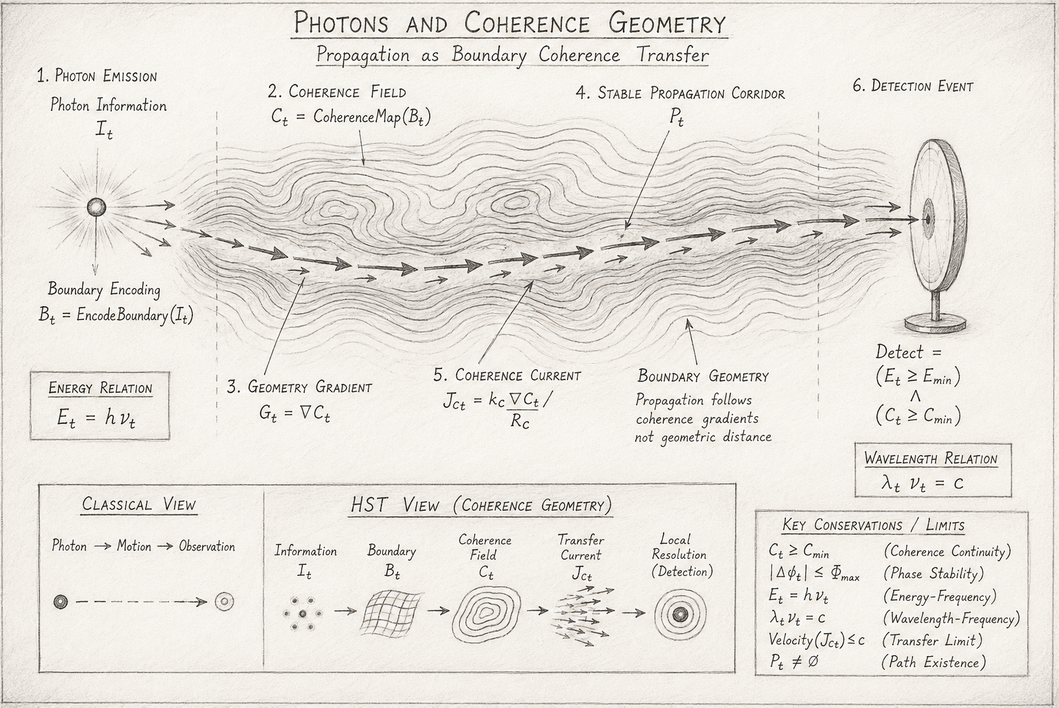
Photons and Coherence Geometry: Propagation as Boundary Coherence Transfe

Overview

This diagram illustrates the Holographic Space-Time (HST) interpretation of photon propagation. Rather than depicting a photon as a fundamental particle travelling through an independent spacetime background, the figure represents light as a coherence-transfer process occurring across an encoded boundary geometry.

The diagram is organised from left to right, following the complete propagation sequence from emission, through coherence formation and transfer, to eventual detection.

The central objective of the figure is to demonstrate that the observable behaviour of photons can be interpreted as the movement of organised coherence through a dynamically evolving boundary field rather than the motion of a discrete particle through empty space.

Telephone:
01377 236594

Photon Emission Region

The left-hand side of the diagram represents the origin of a photon event.

The point source labelled:

\[ I_t \]

corresponds to the initial photon information state.

This state contains all information required for propagation, including:

  • Energy
  • Frequency
  • Phase
  • Polarisation
  • Emission conditions

Within HST, the photon does not begin as a travelling particle.

Instead, it begins as an informational boundary condition that must first be encoded into the surrounding geometric structure.

The emission source therefore represents the initiation of a coherence event rather than the launch of a physical object.

Boundary Encoding

Directly beneath the emission source appears:

\[ B_t = \mathrm{EncodeBoundary}(I_t) \]

This stage represents the conversion of photon information into a physical boundary representation.

The encoded boundary serves as the substrate upon which all subsequent coherence structures emerge.

In HST, physical reality is treated as an evolving boundary system.

The photon therefore becomes a feature of boundary organisation rather than an independent entity existing separately from the geometry.

This operation establishes the initial conditions required for propagation.

Coherence Field Formation

The large central region of the diagram contains numerous contour-like structures labelled:

\[ C_t = \mathrm{CoherenceMap}(B_t) \]

These contours represent the coherence field generated from the encoded boundary state.

The field describes how strongly neighbouring regions of the boundary remain organised relative to one another.

The contour structure is intentionally drawn in a form resembling topographic maps.

This reflects the interpretation that coherence possesses geometry.

Regions of high coherence correspond to stable propagation environments, while regions of lower coherence become increasingly unsuitable for transfer.

The field therefore acts as the geometric landscape through which propagation occurs.

Geometry Gradient Structure

Within the coherence field the diagram identifies:

\[ G_t = \nabla C_t \]

These gradients represent local changes in coherence density.

The gradients determine:

  • Preferred transfer directions
  • Propagation stability
  • Available transfer routes
  • Geometric constraints

Rather than assigning a trajectory to a photon beforehand, the geometry itself determines which routes become available.

This is a central distinction between the HST interpretation and conventional particle-based descriptions.

Propagation follows coherence structure.

It does not define it.

Stable Propagation Corridor

Running through the centre of the diagram is a highlighted corridor composed of directional arrows.

This region is labelled:

\[ P_t \]

and represents the stable path set.

The path emerges naturally from the coherence landscape.

It is not externally imposed.

The corridor indicates regions where coherence remains above the minimum stability threshold:

\[ C_t \geq C_{\min} \]

Within HST, photon trajectories correspond to stable coherence corridors through the boundary geometry.

The route exists because the geometry permits stable transfer.

The photon does not independently select a direction.

The geometry itself determines the available propagation pathway.

Coherence Current

Along the stable corridor are multiple smaller arrows representing the coherence current:

\[ J_{C_t} = \frac{R_C\,k_C\,\nabla C_t}{R_c} \]

This current forms the primary propagation mechanism of the model.

The arrows do not represent particles moving through space.

Instead, they indicate the transfer of organised coherence between neighbouring boundary regions.

The coherence current performs the role conventionally assigned to particle motion.

Information is transferred.

The geometry evolves.

Observable propagation emerges from the interaction of both processes.

Boundary Geometry Distortion

The subtle curvature visible throughout the contour field represents variations in boundary geometry.

These distortions illustrate that propagation follows coherence gradients rather than simple geometric distance.

The figure intentionally demonstrates that the shortest path is not necessarily the physically realised path.

Instead, photons propagate along routes that maximise coherence stability.

This provides an intuitive visual interpretation of phenomena such as:

  • Refraction
  • Gravitational lensing
  • Fibre-optic guidance
  • Curved photon trajectories

Within HST, these effects emerge from changes in coherence geometry rather than forces acting upon moving particles.

Detection Event

The detector shown on the right side of the diagram represents the final stage of propagation.

The associated condition is:

\[ \mathrm{Detect} = (E_t \geq E_{\min}) \;\wedge\; (C_t \geq C_{\min}) \]

Detection occurs when both energy and coherence thresholds are satisfied.

This stage corresponds to the localisation of an otherwise distributed coherence structure.

The diagram therefore illustrates a key HST principle:

During propagation, the photon behaves as a distributed coherence process.

During detection, that coherence resolves into a local interaction.

The apparent particle-like behaviour of photons emerges only at the point of localisation.

Energy–Frequency Relation

The left annotation panel contains:

\[ E_t = h\nu_t \]

This equation preserves the experimentally verified relationship between energy and frequency.

Within HST, the equation is interpreted as a property of the coherence structure itself.

Energy becomes a measurable characteristic of organised coherence rather than a property carried by a fundamental particle.

The diagram therefore remains consistent with quantum observations while reinterpreting their underlying physical meaning.

Wavelength–Frequency Relation

The right annotation panel contains:

\[ \lambda_t \nu_t = c \]

This relation links wavelength and frequency through the maximum coherence transfer rate.

Within the HST framework:

  • Frequency represents boundary update rate.
  • Wavelength represents coherence-cycle spacing.
  • c represents the maximum stable transfer velocity.

The equation therefore describes the geometry of propagation rather than the behaviour of a wave moving through empty space.

Classical Versus HST Interpretation

The lower panel provides a direct comparison between conventional and HST viewpoints.

Classical Interpretation

Photon→Motion→Observation

The photon is assumed to exist as an object that moves through space before being detected.

HST Interpretation

Information→Boundary→
Coherence Field→
Transfer Current→Local Resolution

Here, the photon emerges from a sequence of coherence transformations.

Motion becomes an emergent consequence of transfer rather than a fundamental property.

The comparison highlights the shift from object-based physics to coherence-based physics.

Conservation and Stability Conditions

The lower-right panel summarises the invariants governing propagation.

These include:

\[ C_t \geq C_{\min} \]

for coherence continuity,

\[ \left| \Delta \phi_t \right| \leq \Phi_{\max} \]

for phase stability,

\[ E_t = h\nu_t \]

for energy conservation,

\[ \lambda_t \nu_t = c \]

for propagation geometry,

and

\[ \mathrm{Velocity}(J_{C_t}) \leq c \]

for the universal transfer limit.

Together these conditions ensure that the coherence structure remains physically stable throughout propagation.

Scientific Interpretation

The complete diagram presents photons as stable coherence structures propagating through an evolving boundary field.

The contour geometry represents the organisation of the coherence landscape.

The propagation corridor represents the emergence of stable transfer pathways.

The coherence current represents information transfer between neighbouring regions.

The detector represents the localisation of distributed coherence into an observable event.

Viewed as a whole, the figure provides a visual summary of the HST proposition that light is not fundamentally a particle moving through spacetime but a dynamically maintained coherence process whose observable behaviour emerges from the geometry of information encoded on physical boundaries.

Diagram → Flow Mapping Table

Figure 40.1 — Photons and Coherence Geometry
Diagram Element Visual Representation Flow Component Mathematical Representation Physical Meaning
Photon Source Left-side emission point Photon Information Input I_t Initial photon information state
Emission Arrows Small outward arrows from source Information Transfer Initiation I_t → B_t Beginning of boundary encoding
Boundary Encoding Region Source-to-field transition zone Boundary Encoding B_t = EncodeBoundary(I_t) Converts photon information into boundary structure
Coherence Contours Layered contour field Coherence Field Generation C_t = CoherenceMap(B_t) Creates propagating coherence landscape
Field Density Variations Thick and thin contour spacing Coherence Distribution C_t Represents local coherence strength
Gradient Direction Contour deformation patterns Geometry Gradient Formation G_t = ∇C_t Determines transfer direction
Stable Corridor Dark central pathway Stable Path Construction P_t = {x ∈ B_t | C_t(x) ≥ C_min} Defines physically viable propagation routes
Propagation Arrows Arrow chain through corridor Transfer Update x_t+1 = Transfer(x_t,J_C_t,P_t) Advances coherence through geometry
Coherence Current Arrows Small arrows inside corridor Coherence Current Formation J_C_t = (k_C∇C_t)/R_C Information transfer mechanism
Curved Field Structure Distorted contour lines Geometry Evolution G_t = ∇C_t Demonstrates coherence-guided propagation
Boundary Geometry Region Entire contour landscape Coherence Geometry (C_t,G_t,P_t) Encoded physical structure
Detector Right-side detection plate Detection Resolution Detect = (E_t ≥ E_min) ∧ (C_t ≥ C_min) Localisation of coherence event
Detection Target Detector centre point Photon Localisation Detect Observable photon interaction
Energy Annotation Box Left-side equation panel Energy Conservation E_t = hν_t Energy-frequency coupling
Wavelength Annotation Box Right-side equation panel Wavelength Constraint λ_tν_t = c Coherence cycle geometry
Classical View Panel Lower-left comparison box Conventional Interpretation Photon → Motion → Observation Standard particle description
HST View Panel Lower-centre comparison box Full HST Execution Chain I_t → B_t → C_t → J_C_t → Detect Coherence-based propagation model
Conservation Panel Lower-right invariant box Invariant Monitoring C_t ≥ C_min, Velocity(J_C_t) ≤ c Stability enforcement

Flow Sequence Mapping

Diagram Region Flow Stage Equation
Photon Source Information Input I_t
Boundary Interface Boundary Encoding B_t = EncodeBoundary(I_t)
Coherence Landscape Coherence Generation C_t = CoherenceMap(B_t)
Contour Structure Gradient Formation G_t = ∇C_t
Stable Corridor Path Selection P_t = {x ∈ B_t | C_t(x) ≥ C_min}
Corridor Arrows Coherence Current J_C_t = (k_C∇C_t)/R_C
Transfer Route Propagation Update x_t+1 = Transfer(x_t,J_C_t,P_t)
Detector Local Resolution Detect = (E_t ≥ E_min) ∧ (C_t ≥ C_min)

Geometry Interpretation Mapping

Diagram Feature HST Interpretation Governing Equation
Contour Lines Coherence Topology C_t = CoherenceMap(B_t)
Contour Curvature Boundary Geometry G_t = ∇C_t
Corridor Centreline Stable Transfer Route P_t
Arrow Chain Coherence Transport J_C_t
Detector Impact Point Coherence Resolution Detect
Contour Density Local Coherence Magnitude C_t
Corridor Stability Path Viability C_t ≥ C_min
Geometric Distortion Curvature Effects ∇C_t ≠ 0

Photon Property Mapping

Diagram Component Photon Property Equation
Source Brightness Energy State E_t
Wave-Like Contours Distributed Coherence C_t
Directional Arrows Propagation Direction G_t
Corridor Width Path Stability C_t ≥ C_min
Detection Spot Localisation Event Detect
Energy Box Quantum Energy Relation E_t = hν_t
Wavelength Box Propagation Geometry λ_t ν_t = c
Stability Box Physical Constraints Invariants

Classical ↔ HST Comparison Mapping

Diagram Component Photon Property Equation
Source Brightness Energy State E_t
Wave-Like Contours Distributed Coherence C_t
Directional Arrows Propagation Direction G_t
Corridor Width Path Stability C_t ≥ C_min
Detection Spot Localisation Event Detect
Energy Box Quantum Energy Relation E_t = hν_t
Wavelength Box Propagation Geometry λ_t ν_t = c
Stability Box Physical Constraints Invariants

Complete Figure Execution Chain

It​→Bt​→Ct​→Gt​→
Pt​→JCt​​→xt+1​→Bt+1​→
Detect


Figure Summary Statement

The diagram represents the complete HST photon propagation sequence.

The emission source corresponds to photon information input, the contour field represents the generated coherence geometry, the central corridor represents stable propagation pathways, the arrow chain represents coherence current transfer, and the detector represents local coherence resolution.

Every visual element maps directly to a corresponding Flow Algebra operation, creating a one-to-one correspondence between geometry, execution logic, and mathematical representation.

Execution Guarantee Statement

Photons and Coherence Geometry

Execution Guarantee

The Photons and Coherence Geometry Flow is guaranteed to execute successfully if and only if all coherence, phase, energy, and propagation constraints remain satisfied throughout the complete boundary-transfer cycle.

Execution success does not depend upon the existence of a travelling particle. Instead, successful execution requires the preservation of a stable coherence structure capable of transferring encoded information across neighbouring boundary regions.

The flow guarantees that photon propagation will occur whenever a valid coherence field, stable transfer pathway, and physically permissible transfer current simultaneously exist.

Formally:

Execution(Photont​)=SUCCESS

if

\[ C_t \geq C_{\min} \]

and

\[ \left| \Delta \phi_t \right| \leq \Phi_{\max} \]

and

\[ P_t \neq \emptyset \]

and

\[ \mathrm{Velocity}(J_{C_t}) \leq c \]

and

\[ E_t \geq E_{\min} \]

Guaranteed Boundary Encoding

For every valid photon information state:

\[ I_t \]

the flow guarantees construction of a corresponding boundary state:

\[ B_t = \mathrm{EncodeBoundary}(I_t) \]

provided the information state remains physically defined.

Thus no valid photon state enters propagation without first producing a boundary representation.


Guaranteed Coherence Generation

For every valid boundary state:

\[ B_t \]

the flow guarantees generation of a coherence field:

\[ C_t = \mathrm{CoherenceMap}(B_t) \]

ensuring that propagation always occurs within a well-defined geometric structure.

No propagation stage can execute without coherence geometry first being established.

Guaranteed Gradient Formation

Given a valid coherence field:

\[ C_t \]

the flow guarantees calculation of:

\[ G_t = \nabla C_t \]

thereby providing the directional information required for propagation.

Direction emerges automatically from coherence geometry and requires no external path assignment.

Guaranteed Path Construction

The flow guarantees formation of a stable propagation route whenever coherent regions remain available:

\[ P_t = \left\{ x \in B_t \;\middle|\; C_t(x) \geq C_{\min} \right\} \]

If at least one coherent region exists, at least one propagation route exists.

Formally:

\[ C_t \geq C_{\min} \;\Rightarrow\; P_t \neq \emptyset \]

Guaranteed Phase Preservation

The flow guarantees preservation of interference structure and wave behaviour whenever:

\[ \left| \Delta \phi_t \right| \leq \Phi_{\max} \]

Under this condition:

  • Phase continuity remains intact.
  • Interference remains physically meaningful.
  • Wave coherence remains stable.
  • Propagation proceeds without decoherence.

Guaranteed Energy Conservation

The flow guarantees maintenance of the photon energy relation:

\[ E_t = h\nu_t \]

throughout execution.

No propagation update may violate this constraint.

Energy remains coupled to frequency at every stage of transfer.

Guaranteed Wavelength Consistency

The flow guarantees maintenance of the propagation geometry constraint:

\[ \lambda_t \nu_t = c \]

throughout all transfer updates.

This ensures that coherence spacing and update rate remain physically compatible.

Guaranteed Transfer Stability

The coherence current:

\[ J_{C_t} = \frac{R_C\,k_C\,\nabla C_t}{R_c} \]

is guaranteed to remain physically stable whenever:

\[ \mathrm{Velocity}(J_{C_t}) \leq c \]

Under this condition:

  • Information transfer remains coherent.
  • Boundary continuity remains intact.
  • Propagation remains physically realizable.

Guaranteed Boundary Evolution

For every successful propagation step:

\[ x_{t+1} = \mathrm{Transfer} \!\left( x_t,\, J_{C_t},\, P_t \right) \]

the flow guarantees a corresponding geometric update:

\[ B_{t+1} = \mathrm{UpdateBoundary} \!\left( B_t,\, x_{t+1},\, E_t,\, \phi_t \right) \]

ensuring that propagation and geometry evolve together.

No successful transfer occurs without updating the boundary state.

Guaranteed Detection

The flow guarantees localisation whenever:

\[ (E_t \geq E_{\min}) \;\wedge\; (C_t \geq C_{\min}) \]

is satisfied.

Formally:

Detect=TRUE

Under these conditions the distributed coherence structure resolves into an observable photon event.

Failure Conditions

Execution is guaranteed to terminate if any of the following occur:

Coherence Collapse

\[ C_t < C_{\min} \]

Phase Decoherence

\[ \left| \Delta \phi_t \right| > \Phi_{\max} \]

Path Elimination

\[ P_t = \emptyset \]

Transfer Limit Violation

\[ \mathrm{Velocity}(J_{C_t}) > c \]

Detection Threshold Failure

\[ E_t < E_{\min} \]

Any such condition produces:

\[ \mathrm{Execution}(\mathrm{Photon}_t) = \mathrm{FAIL} \]

Deterministic Execution Guarantee

The complete propagation chain:

It​→Bt​→Ct​→Gt​→Pt​→JCt​​→xt+1​→Bt+1​→Detect

is fully deterministic.

For identical inputs, identical boundary conditions, identical coherence geometry, and identical physical parameters, the flow will always produce the same propagation outcome.

No probabilistic execution step is required by the flow itself.

Formal Guarantee Statement

\[ (C_t \geq C_{\min}) \;\wedge\; \left( \left| \Delta \phi_t \right| \leq \Phi_{\max} \right) \;\wedge\; (P_t \neq \emptyset) \;\wedge\; \left( \mathrm{Velocity}(J_{C_t}) \leq c \right) \;\wedge\; (E_t \geq E_{\min}) \]

⟹

Execution(Photont​)=SUCCESS


Scientific Interpretation

Under the HST framework, photon propagation is guaranteed whenever a stable coherence structure can be maintained across the boundary geometry.

The flow therefore guarantees that light emerges as a coherent transfer process, preserving phase, energy, wavelength relations, and localisation behaviour, while remaining fully constrained by the geometry of the underlying coherence field.

Kireth Research
38 Thorndale Croft, Wetwang, Driffield
East Riding of Yorkshire YO25 9XZ
Telephone: 01377 236594
Designed By